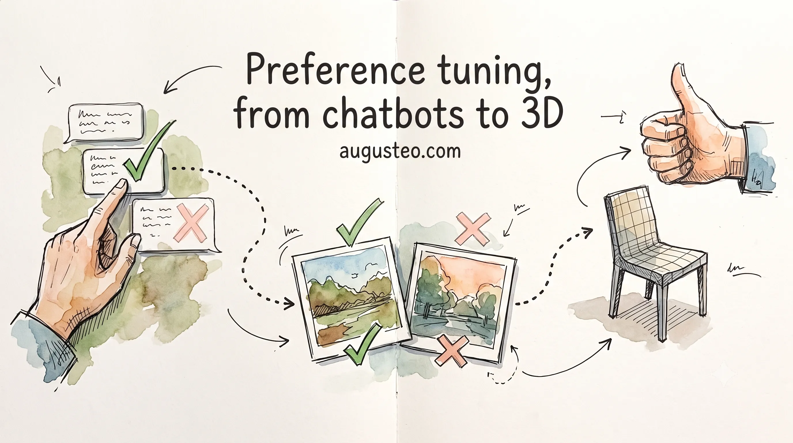
Preference tuning, from chatbots to 3D

Preference tuning is how you train a model on “this one, not that one” instead of “copy this.” It grew up in chatbots, as RLHF and then DPO and GRPO, and it has quietly become the data engine behind Meta’s SAM 3D. This post follows a single human verdict the whole way: from a chatbot A/B click to a verdict on a reconstructed 3D shape. Written for engineers who know deep learning and fine-tuning but not much reinforcement learning. About a 30-minute read.

1. The thing you can’t demonstrate

Supervised fine-tuning teaches by example. You hand the model a prompt and the answer you want, and it learns to copy. That works as long as you can write the answer down.

For a lot of what we now ask models to do, that gets expensive fast. Someone can write an acceptable reply to “explain recursion to a nervous beginner,” but nobody can author the best one. Nobody can paint the one correct image for “a cozy reading nook, golden hour.” Nobody can hand-model the exact 3D mesh of the chair in a photo. Imitation still works here, and every system in this post uses it, but each demonstration costs an expert’s time and none of them tells the model which of two attempts you would rather have. “Good” past that ceiling is a matter of taste, and taste doesn’t come as a worked example.

But you can do something easier. Show a person two answers and they will tell you which is better. They can’t write the perfect summary, but they can point at the better of two summaries in a second. That gap, between what people can produce and what people can judge, is the whole reason preference tuning exists. It is a way to train on judgments instead of demonstrations: on “this one, not that one.”

The verdict is the unit we are going to follow. In a chatbot it is a labeler clicking the better of two replies. By the end of this post it is an annotator looking at a 3D shape a model reconstructed from a photo and rating how good it is. Same verdict, same math underneath, worlds apart in what it builds. The trip from one to the other is the post.

Act 1 — From a click to a loss

How a single “A beats B” becomes a number a model can train on, and the two ways the field learned to use it.

2. Turning a verdict into a number

A raw verdict is binary: A won, B lost. Gradient descent can’t do much with one bit. To train on preferences you need to turn “A beats B” into a smooth quantity you can push on.

The trick is older than deep learning. In 1952 the statisticians Ralph Bradley and Milton Terry wrote down a model for exactly this: give each item a hidden score, and say the probability that A beats B is the logistic function of the gap between their scores. The logistic function, also called the sigmoid, is just the S-shaped curve in Fig 2: hand it any score gap, however large or negative, and it squashes it into a probability between zero and one. If the scores are equal, the gap is zero and it returns a coin flip. As A’s score pulls ahead, the probability A wins slides up toward one; as it falls behind, down toward zero.

That single curve is the seed of everything that follows. Every method here that turns a verdict into a training signal, the reward model in the next section and the DPO family after it, is underneath a way of assigning scores so that the better answer gets the higher one, with the Bradley-Terry sigmoid converting the score gap into “how confident are we that this was the right call.” (The policy-gradient methods later in the post, GRPO and its successors, sit downstream of a reward and have no sigmoid in them; that distinction matters and section 5 comes back to it.) Hold onto the shape: small gap, near 50/50; large gap, near certain. When we get to the loss functions, that sigmoid is the part doing the work.

3. The first recipe: RLHF and PPO

The recipe that made preference tuning a standard tool was InstructGPT, OpenAI’s instruction-following work (building on an earlier clean result, Stiennon et al’s reward-model-beats-the-metric finding on summarization in 2020). Its method, reinforcement learning from human feedback, has three stages. Because the rest of the post leans on every piece of it, here is the whole vocabulary, one rung at a time.

Start with the SFT model: a base model fine-tuned on demonstrations. This is the model we improve, and, importantly, the model we keep measuring everything against later. Call it the reference.

Stage two trains a reward model: a learned judge. You collect comparisons, where a labeler picks the better of two model outputs, and you train a network to predict those picks. It is the human’s taste, distilled into something you can call cheaply, at whatever scale training needs. Under the hood it scores each output and fits the Bradley-Terry sigmoid from the last section to the human’s choices.

Stage three is the reinforcement learning. The model produces answers (a rollout, just the model trying things), the reward model scores them, and you nudge the model toward higher-scoring answers. Two more pieces make this work. A critic is a second network that guesses, for a half-finished answer, how good the final score is likely to be; the advantage is then how much better an answer did than the critic expected, the extra credit beyond the baseline. And a KL leash: a penalty for drifting too far from the SFT reference. KL is the Kullback-Leibler divergence, a standard measure of how far apart two probability distributions are, and here it measures how far the model’s word-by-word probabilities have moved from the reference’s, so penalizing it is what keeps the model tethered. You need the leash because a model chasing reward with none will find some degenerate text the reward model loves and normal readers hate. InstructGPT says it plainly: “we add a per-token KL penalty from the SFT model at each token to mitigate over-optimization of the reward model.” The optimizer that takes the step is PPO, short for Proximal Policy Optimization, a standard reinforcement-learning algorithm. “Proximal” is the whole idea: for each token it samples, the objective clips the ratio between the new model’s probability for that token and the old model’s, which, as the PPO paper puts it, “removes the incentive for moving” that ratio outside a narrow interval. Nothing forcibly holds the weights in place; the reward for wandering is simply cut off.

It worked, and the headline result is still striking: a 1.3B-parameter InstructGPT model’s answers were preferred over those of 175B GPT-3, a model more than a hundred times larger. On that comparison the preference-tuned small model simply won.

It also cost a lot. You are training two extra networks, a reward model and a critic (the critic about as big as the policy), and sampling fresh rollouts every step. And the whole RL loop is fiddly enough that the people who came next described their main selling point as not having to do it.

4. The shortcut: DPO

Direct Preference Optimization came from a sharp observation in its 2023 paper, captured in its subtitle: your language model is secretly a reward model. The full RLHF objective, maximize reward while staying near the reference, has a known closed-form optimum, and you can run the algebra backwards. When you do, the reward drops out and you are left with a quantity the model already computes: the log-ratio of how likely the model is to produce an answer versus how likely the reference is.

Unpack that phrase, because the whole method rests on it. The ratio is just “how many times more likely”: if the model is twice as likely as the reference to produce the answer, the ratio is two; if half as likely, the ratio is one-half. Taking the log of it turns that into a tidy signed number, zero when the two agree, positive when the model favors the answer more than the reference does, negative when less (the ratio of two becomes about +0.7, the one-half becomes about −0.7). So the log-ratio is a single number that says, in one direction or the other, how far the model has moved away from the reference on this particular answer.

Here is what falls out. The implicit reward of an answer is β (beta, a single tuning knob we look at on its own in a moment) times that log-ratio, written log(π/π_ref), plus a constant that depends only on the prompt and cancels the moment you compare two answers to it, where π (pi) is the probability the model you are training assigns to the answer and π_ref is the frozen SFT reference’s probability. So you do not need a separate reward model, and you do not need the RL loop at all. You take your preference pairs, drop them straight into the Bradley-Terry sigmoid using that implicit reward, and train with one ordinary classification loss. The DPO paper’s words: it works “without explicit reward modeling or reinforcement learning,” and is “computationally lightweight, eliminating the need for sampling from the LM during fine-tuning or performing significant hyperparameter tuning.”

Written out, the loss is a single line, and every term earns its place. Fig 5 lays it out with each piece labeled. The outer sigmoid is the Bradley-Terry curve from section 2; inside it sits the difference of two log-ratios, how much more the model favors the winning answer than the frozen reference does, minus the same for the loser. Push that difference up and the loss falls. The frozen SFT model appears in both terms as the yardstick you are measured against. And β is a knob we need to look at on its own.

4½. The β leash, and which way it points

β is the same leash from RLHF, now living inside the DPO loss, and it is easy to get backwards, so here it is carefully. β controls how far the model is allowed to drift from the reference. A high β is a strong leash: the model stays close to the SFT model and moves only a little. A low β is a loose leash: the model is free to wander far from the reference to fit the preference data harder, and with it comes the risk of overfitting the comparisons and degrading.

The direction surprises people because “higher” sounds like “more aggressive.” It isn’t. The implicit reward is β times the log-ratio, so a higher β means even a small change in the model’s probabilities produces a large reward signal, and the model reaches the same preference margin with less movement. More β, less drift. The DPO paper states it as “β is a parameter controlling the deviation from the base reference policy.”

5. Dropping the critic: GRPO

DPO removed the reward model and the RL loop. The other big simplification went the other way, keeping the RL loop but cutting the critic, and it is worth being precise about where it sits. Group Relative Policy Optimization, introduced in DeepSeek’s DeepSeekMath, is not a way to turn a verdict into a reward. It assumes a reward already exists and is a cheaper way to estimate the advantage from section 3.

Recall the critic: a second network, about the size of the policy, whose only job is to guess the baseline an answer should beat. GRPO deletes it. Instead of learning a baseline, it samples a whole group of answers to the same prompt, scores them all, and uses the group’s average score as the baseline. An answer’s advantage is then how much it beat its siblings, divided by how spread out their scores were so every group lands on a comparable scale. (That last division looks harmless here; section 13 shows where it bites.) The DeepSeekMath figure caption is blunt about the payoff: GRPO “foregoes the value model, instead estimating the baseline from group scores, significantly reducing training resources.”

Because GRPO sits downstream of the reward, the reward can be anything. In DeepSeek-R1, the reasoning model GRPO trained (peer-reviewed in Nature in 2025), the reward is often a plain rule: did the math answer come out correct? No human preferences, no reward model, just a checker. That is the cleanest illustration of the split this post keeps drawing: where the reward comes from is one decision, and how you estimate advantage from it is a separate one. Bradley-Terry and DPO are about the first. GRPO is about the second.

6. Where the verdict is not enough

It would be easy to read this far and conclude that preference tuning is a clean win that keeps getting cleaner. It isn’t, and a post that pretended otherwise would be lying by omission. Three honest caveats.

DPO is not strictly better than the RL loop it replaces. A careful 2024 study found that “DPO may have fundamental limitations” and that PPO-style RLHF, run properly, “is able to surpass other alignment methods in all cases” on their benchmarks, including the hard ones. The shortcut is cheaper and often good enough, not universally superior.

Which method wins is not even fixed. A 2025 analysis showed that “RLHF, DPO, or online DPO can outperform one another depending on type of model mis-specifications,” and that when the reward is sparse, the two-stage RLHF route can need far fewer samples than DPO to find a good model. The right answer is “it depends on your setup,” which is unsatisfying and true.

And GRPO has its own pathologies. One 2025 paper identified an optimization bias that “artificially increases response length (especially for incorrect outputs),” the model learning to ramble because the math rewards it; another found GRPO “vulnerable to reward hacking, optimizing only one of the objectives at the cost of the others.” None of this sinks preference tuning. It just means the verdict is a powerful signal, not a magic one.

Act 2 — The crossover to vision

The same verdict, the same loss, now pointed at pixels and shapes instead of tokens.

7. The same verdict, now on images

Everything so far has been about language, where an answer is a sequence of tokens and the model assigns each one a probability. The DPO loss leaned hard on that: it needs the model’s likelihood of the winning answer and the losing answer, the π(win) and π(lose) in the equation. An image generator does not produce tokens with neat probabilities. So how do you plug a picture into a loss built for log-probabilities?

The bridge is Diffusion-DPO, and it is worth walking in steps because the jump is where intuition usually breaks.

1. DPO needs a likelihood ratio for the winning and losing outputs.
2. An image generator has no token log-probs to supply one.
3. But a diffusion model does expose a stand-in for likelihood: the training objective itself, the denoising loss that measures how well the model reconstructs an image along its noising trajectory. You cannot read off the exact probability a diffusion model assigns to a finished image, the way you can multiply token probabilities for a sentence, but you can compute a quantity that bounds it. The denoising loss is the computable piece; flip its sign and you have the ELBO (evidence lower bound), a number that stays underneath the log-likelihood you wish you could evaluate. Driving the denoising loss down pushes that bound up, which is all the loss needs.
4. Diffusion-DPO puts that denoising term where DPO’s token log-likelihood sat. Getting there is more than a substitution, since the paper has to bound an objective defined over whole noising paths before a tractable difference of denoising losses falls out, but the loss you end up training on has the shape of the DPO loss with a denoising term inside it.

The skeleton, winner over loser measured against a frozen reference, survives intact. What the loss actually pushes on is the gap: the winner’s trajectory has to gain on the reference by more than the loser’s does. Neither image has to move in an absolute direction on its own.

It works in practice. Diffusion-DPO reports training on 851,000 crowdsourced preference pairs drawn from the Pick-a-Pic dataset of human choices over generated images, and tuned Stable Diffusion XL until it “significantly outperforms” the base model on human preference for both visual appeal and prompt-faithfulness. It is the same kind of generator that image generators are quietly becoming the best vision models and the generative vision stack put at the center of perception; preference tuning is how you give that generator taste.

One subtlety worth flagging, because it is where the vision story stops being a copy of the language story. The plain sigmoid loss, designed for the clean “this token, not that token” world, turns out to be a slightly awkward fit for the smooth, regression-like job of generating an image. A 2026 paper on flow-matching generators argues that standard DPO’s margin-maximization behavior “is fundamentally ill-suited for the regression nature of diffusion and flow-matching models.” The verdict still crosses over. It just doesn’t land quite the same way.

8. A cheap verdict beats authoring the answer

Step back from the loss and look at the data. The expensive part of a vision dataset has always been authoring the target: tracing a segmentation mask by hand, modeling a 3D mesh, labeling every pixel. The cheap part is judging a model’s attempt. And that asymmetry is the whole reason preference tuning matters for vision data, not just vision models.

This data-collection idea is older than the preference-tuning machinery, and it is worth being clear that it is a separate idea: not a training method like DPO, just a cheaper way to gather labels. It showed up in plain 2D segmentation, with no reinforcement learning anywhere in it. A 2022 study replaced mask-drawing with annotation “where only point-wise yes/no questions are answered,” and scaled it to 22.6 million point labels across 4,171 classes. The annotators never drew a boundary; they answered a model’s yes/no questions. That is the same shape as the verdict from Act 1, “this one, not that one,” now pointed at building a dataset instead of training a model directly: don’t make the human author the answer, make the model propose and the human give a cheap verdict. Hold onto that distinction, because the next section wires the two back together.

This is the shape that segmentation models like the ones in the unified vision stack are built to consume, and it is exactly the bet SAM 3D makes for 3D. As the team puts it in Meta’s SAM 3D writeup, “verifying or ranking meshes is a more accessible skill” than building them, so the team “can thus scale by building a data engine asking annotators to rate multiple options generated by a suite of models in the loop.” In her CVPR 2026 talk on the work, Georgia Gkioxari put the annotator’s job even more bluntly: they only say yes or no. A non-expert can do it, which is the point: the verdict is cheap enough to collect at the scale a foundation model needs.

9. The model-in-the-loop data engine

A cheap verdict is only powerful if you wire it into a loop. The loop is the idea, going back to the original Segment Anything model, that the model and the dataset can improve each other. The model proposes labels; humans verify or correct them; the corrected labels retrain the model; the better model makes better proposals, so the humans correct less and approve more. SAM’s loop produced over 1 billion masks across 11 million images, a dataset no team could have drawn by hand.

By 2026 the loop has a new wrinkle: the model does some of the verifying too. SAM 3 uses multimodal language models as “AI annotators” and then fine-tunes them into “AI verifiers that achieve near-human accuracy,” which more than doubles annotation throughput over a human-only pipeline. Models now sit on both sides of the loop: SAM 3 proposes the masks, language models propose the concepts to label, and separately fine-tuned models check the results. The verdict didn’t disappear. It got partly automated.

10. The climax: SAM 3D

Now put every piece together, because SAM 3D is where they all meet. The problem is a data gap with no easy way around it: SAM 3D reconstructs the full 3D shape, texture, and pose of an object from a single ordinary photo, and there is no way to crowdsource 3D ground truth for real photos. You cannot ask a worker to hand-model the chair in a snapshot. The team calls its answer breaking the 3D “data barrier.”

Their answer is the whole post in one system. Start with synthetic pretraining, a flood of computer-generated 3D scenes, the way you might pretrain on cheap data before fine-tuning on the real thing, which is the same instinct behind picking the right pretraining recipe for out-of-distribution data. Then align the model to reality using the cheap verdict: the team collects training samples and preference data from humans and uses them, in the paper’s words, “in both supervised finetuning (SFT) and direct preference optimization (DPO).” That is the same preference-optimization pattern from section 4, adapted to a 3D generator the way Diffusion-DPO adapted it to images, with the winning mesh as the chosen output and a worse one as the rejected. And it is a loop: that alignment step “can be repeated,” each round’s better model generating better mesh proposals for the next round of cheap human verdicts.

The engine ran on almost 1 million images and produced roughly 3.14 million meshes, and the model it trained wins decisively: in head-to-head human preference tests against prior work, SAM 3D reports “at least a 5:1 win rate in human preference tests on real-world objects and scenes.” The team tracks quality with Elo, the chess rating, where “a 400 point Elo difference corresponds to 10:1 odds in a preference test,” and reports that the rating keeps climbing as the data engine runs more rounds. The throughline has arrived at its destination. The same verdict that picked the better chatbot reply, “this one, not that one,” picked the better 3D mesh, and enough of those verdicts, looped through a model that proposes and a human who judges, added up to a 3D foundation model.

Coda

11. The frontier, part one: GSPO

Three threads run past the methods in this post, and all three are the same throughline pushed one notch further. The first is a repair to GRPO.

Recall that GRPO, like PPO, reuses each batch of sampled answers for several gradient steps, because sampling answers from the model is the expensive part. The catch is that after the first step the model has already shifted, so those answers were drawn from a version of the model that no longer exists. The standard fix is importance sampling: scale each piece of the update by a correction factor, the ratio of how likely the current model is to produce that piece to how likely the old model was. Twice as likely now, count it double; half as likely, count it half. It is the bookkeeping that corrects for the mismatch, approximately, so slightly stale samples stay usable.

The Qwen team’s GSPO, Group Sequence Policy Optimization, traces GRPO’s training instability to where that correction is applied. The two names sit one word apart, and so do the methods. GRPO is group relative: it scores each answer against its siblings. GSPO keeps that group baseline exactly as it is and changes only the granularity of the importance ratio, from the token to the sequence. One correction for the whole answer instead of one per word. Everything else in this section follows from that single move.

GRPO computes the ratio per token, one for every word in the answer, and applies it to that token’s own slice of the loss. The trouble, in the paper’s words, is that “since this weight is based on a single sample from each next-token distribution, it fails to perform the intended distribution-correction role.” A single noisy ratio on a single token is survivable. Hundreds of them, each a wild one-sample estimate, scattered across a long answer and then each run through the clip is not. The paper describes “high-variance training noise that progressively accumulates with increased response length and is further amplified by the clipping mechanism, ultimately precipitating model collapse,” and pins the whole problem on “the fundamental misapplication and invalidation of importance sampling weights.” For mixture-of-experts models, where which experts fire can change between updates, it is worse still.

GSPO’s fix is one observation: “since the reward is granted to the entire sequence, applying off-policy correction at the token level appears problematic.” So it computes a single ratio for the whole answer, “based on sequence likelihood,” and does “sequence-level clipping, rewarding, and optimization.”

It helps to see the two ratios side by side, with each piece labeled. Fig 13 lays them out. GRPO’s correction is one fraction for every token: how likely the current model is to produce that token, over how likely the old model was. If the model has not moved the fraction is one and nothing changes; if the current model likes the token twice as much, the fraction is two. GSPO swaps all of those for a single fraction over the whole answer, raised to the power one over the answer’s length.

That exponent is the quiet workhorse. A sequence’s probability is the product of its token probabilities, so taking the length-th root of the ratio is exactly the geometric mean of the per-token ratios: it folds the whole noisy product into one number on a stable scale, the way the n-th root of a product of n numbers reports their typical size instead of their runaway product. A long answer and a short one now land in a more comparable range, and one freak token has far less pull on the correction. The result, in the team’s words, “notably stabilizes Mixture-of-Experts (MoE) RL training” and “contributed to the remarkable improvements in the latest Qwen3 models.”

Nothing about the verdict changed here. This is the section-5 advantage machinery, corrected at the granularity the reward actually lives at.

GSPO is not the only repair, and the cluster is worth a glance, because each one names a different way naive GRPO breaks. DAPO, Decoupled Clip and Dynamic sAmpling Policy Optimization, names its two headline fixes in its own acronym and is GRPO plus four of them: an asymmetric clip that protects exploration (the decoupling), dynamic sampling that throws out prompts where every answer is right or every answer is wrong, token-level loss, and a soft length penalty. Together they reach “50 points on AIME 2024 using Qwen2.5-32B base model.” MiniMax’s CISPO, Clipped IS-weight Policy Optimization, goes after the clip itself, and as the name says it “clips importance sampling weights rather than token updates,” so a rare but load-bearing reasoning token like “Wait” or “However” keeps contributing a gradient instead of being zeroed out, the same granularity instinct as GSPO aimed at a different symptom. And the length bias from section 6, diagnosed by Dr. GRPO, is a third: delete two of GRPO’s normalizers and the model stops padding wrong answers. Four papers, four different failures of the same algorithm, which is what a method looks like when it is being pushed hard enough to be worth fixing.

12. The frontier, part two: when the critic comes back

The second thread doubles back on the post’s own plot. Read the lineage as a story of throwing machinery away: RLHF ran a reward model, a critic, and a sampling loop; DPO dropped the reward model and the loop; GRPO dropped the critic. Less apparatus at every step. SAO, Single-rollout Asynchronous Optimization, the method used to train GLM-5.2, is where the trend reverses, because one of the hardest new settings cannot afford a piece we deleted. Its name is its argument: one rollout per prompt, trained on the moment it arrives.

The setting is asynchronous agentic RL. When a model is doing long-horizon agentic work, calling tools, writing code, taking many turns, the answers take wildly different times to finish, and a synchronous loop that waits for the whole batch leaves the fast rollouts stalled behind the slowest trajectory. Asynchronous RL removes that stall by “updating the model as rollouts arrive” instead of in locked batches. But that efficiency collides with GRPO. GRPO needs a group of answers to the same prompt to compute its baseline, and, in the paper’s words, “the group has to wait for the slower one to finish before fed into training.” The group is a synchronization barrier bolted onto a pipeline whose whole point was to remove one. Worse, “group-wise sampling is incompatible with online or complex agentic settings where the environment often provides only a single trajectory feedback per prompt”: sometimes there is no group to be had, because the world hands you one attempt and moves on.

So SAO makes the obvious cut: “we replace group-wise sampling with single-rollout sampling, that is, using one rollout per prompt.” One prompt, one answer, straight into training. But that reopens a problem section 5 had closed. GRPO could drop the critic only because the group gave it a baseline, the average score of the siblings. With a single rollout there are no siblings, so there is no group mean, and a bare reward with nothing to compare it against is exactly the high-variance signal that made naive policy gradients unusable. The paper says it plainly: single-rollout optimization “inherently suffers from high variance in gradient estimation, similar to REINFORCE. To reduce variance requires a sufficiently good value model.”

That last sentence is the reversal. The value model is the critic, the second network section 5 celebrated GRPO for deleting. To make single-rollout training work, SAO brings it back. The baseline has now made a full round trip: PPO learned it with a critic, GRPO replaced the critic with a group mean, and SAO, having given up the group, returns to a learned critic. You might ask why not a cheaper stand-in, say a running average of recent rewards, instead of a whole second network. SAO tried exactly that, and it trailed badly (79.8 against 97.3 on AIME 2025). For single-rollout training the learned critic earned its keep.

The reason this is not simply undoing GRPO’s gains is that SAO makes the critic work, which is the part PPO’s critic was bad at. Two tricks do it, and neither is a saving. It updates the value model more often than the policy, “for every single gradient update applied to the policy, we enforce K updates to the value network,” with K set to two, so the critic keeps up with a policy that is moving under it. That is more critic compute, not less, spent on keeping the baseline accurate. And it freezes part of the critic: a “Frozen-Attention” scheme holds the value model’s attention modules fixed and trains only its mixture-of-experts projections, on the finding that the attention layers were the source of the unstable gradients. Fewer trained parameters, but the point is stability rather than economy. The memory bill for a second policy-sized network is still there. What changed is that the critic now earns it.

One more piece connects straight back to the first thread. SAO faces the same off-policy problem GSPO was about, and treats it a different way. Where GSPO moved the importance ratio to the sequence level, SAO stays at the token level GSPO abandoned but drops the separate old-policy term: it “directly uses the log-probabilities from the rollout engine,” and masks any token whose ratio wanders too far outside a strict two-sided band instead of clipping it. The paper notes this is deliberately “simpler by further removing” the old-policy model. Same disease as section 11, off-policy drift, a different cousin of the same medicine.

Does it work? On the paper’s own asynchronous setup, training a Qwen3-30B-A3B model, SAO “is able to train stably for one thousand steps” while “standard GRPO suffers from a performance collapse at approximately 160 training steps,” and it beats the GRPO baselines on both benchmarks: on AIME 2025, 97.3 against 93.5 for the best-tuned GRPO variant and 84.2 for standard GRPO’s last score before it collapsed; on SWE-Bench Verified, 29.8 against 27.0. One caveat kept honest: this is GRPO collapsing in an aggressive asynchronous regime that stresses off-policy drift, not GRPO failing in general. The same GRPO trained DeepSeek-R1 without incident in section 5. The lesson is not that one method dethroned another; it is that the right amount of machinery depends on the setting, and the critic that looked obsolete turns out to be exactly what one of the hardest new settings needed back.

Like GSPO, none of this touched the verdict. This is optimizer-side plumbing, upstream of where the preference signal enters, and SAO’s reward in these experiments is a correctness check, not a human comparison. Of the three frontier stops this is the one furthest from the pairwise verdict the post has been following. The next one runs straight back into it.

13. The frontier, part three: Pref-GRPO closes the loop

The third thread runs through vision, and it ends where the post began.

There is a step to fill in first, because GRPO does not obviously fit an image generator. GRPO is a policy-gradient method: it needs the generator to be a stochastic policy, one that makes a real random choice at every step and assigns each choice a probability it can then nudge up or down, the way a language model assigns a probability to each token it samples. A flow-matching image model, sampled the normal way, is not that. Its sampler is a deterministic ordinary differential equation: fix the starting noise and the path to the finished image is fixed, with no per-step choice to take a gradient through. You can still get a spread of different images by starting from different noise, but you cannot do the step-by-step credit assignment a policy gradient runs on. Flow-GRPO, the paper that first put “online policy gradient reinforcement learning (RL) into flow matching models,” supplies the missing piece with “an ODE-to-SDE conversion that transforms a deterministic Ordinary Differential Equation (ODE) into an equivalent Stochastic Differential Equation (SDE) that matches the original model’s marginal distribution at all timesteps.” In plain terms, it makes each denoising step genuinely random, turning the fixed path into a stochastic policy GRPO can optimize, and it does so “matching the original model’s marginal distribution,” so the images the model produces on average do not change. Now GRPO has something to work on.

With the sampler turned into a policy, the obvious way to run GRPO on images is to sample a group for one prompt, score each image with a reward model, then turn those scores into advantages the section-5 way, by centering and scaling within the group, shown term by term in Fig 17: subtract the group’s average reward from this image’s reward, then divide by the group’s spread. The subtraction is the baseline from section 3; the division is meant to put every group on a comparable scale.

Pref-GRPO shows that the division is exactly the trap. A reward model handed several images for one prompt tends to score them very close together, because they are all reasonable attempts, so the spread is tiny. Standardizing by that spread does not make the advantages enormous, since dividing by the standard deviation lands every group on the same scale by construction. What it does is worse: it promotes a meaningless gap to a full-strength training signal. In the paper’s words, “tightly clustered scores within a group are disproportionately amplified after dividing by the small group standard deviation, driving the policy to over-optimize.” A 7.21 and a 7.19 come out the other side as a confident push toward one image, when the difference is noise and its sign might flip on a rerun. The paper names this the illusory advantage, and it shows where the model goes with it: “scores keep rising while image quality deteriorates, manifesting as oversaturation or unnaturally dark artifacts.” That is plain reward hacking, and the fix is not to clip harder but to change what the reward measures.

The repair is the move this whole post has been about. Instead of asking what score each image gets, Pref-GRPO asks which of two images is better, the same pairwise verdict from section 1. It “reformulates the GRPO objective to pairwise preference fitting”: as the paper puts it, “image pairs within a group are compared by a Pairwise Preference Reward Model (PPRM), and each image’s win rate serves as the reward.” An image’s reward becomes its win rate, the fraction of its group-mates it beats head to head, broken down in Fig 18.

An image that beats every rival scores one; one that loses every time scores zero. Feed those win rates into the same advantage formula and the trap springs open: because win rates spread across the full range from zero to one, a clear winner near one and a clear loser near zero, the spread is genuinely large instead of vanishing. The paper’s reasoning: “because win rates reflect relative rankings rather than absolute scalar scores, Pref-GRPO yields larger within-group variance,” and in their experiments it “produces more stable advantages than pointwise scoring, substantially alleviates reward hacking, and improves semantic alignment.” A preference model can still be wrong, so this is not a guarantee that the verdict is right. It is a reward whose size now tracks something real.

14. Which method for which job

A reader who made it here wants the practical takeaway: which one do I reach for? The honest answer is the through-line of section 6 and section 12. There is no single winner. Every method on this list is the right choice for some setting and the wrong choice for others, and the newest is not the best by default. What follows is a map from setting to method, not a ranking.

Your setting	Reach for	Why, and the catch
A fixed dataset of preference pairs, and you want cheap and stable	DPO	No reward model, no RL loop, one classification loss (section 4). The catch: a well-run PPO can still beat it, and DPO can overfit (section 6).
A reward you can model or a sparse reward signal, and you can afford the loop	PPO-style RLHF	The reward-model-plus-critic pipeline that started it all (section 3). Under a sparse reward it can need far fewer samples than DPO. The catch: two extra networks and a fiddly loop.
Verifiable rule-based rewards (math, code), trained synchronously	GRPO	Drops the critic for a group baseline (section 5); trained DeepSeek-R1. For long sequences or mixture-of-experts, add the stability fixes: GSPO, DAPO, CISPO (section 11).
Asynchronous agentic RL at scale, or online settings with one trajectory per prompt	SAO	Single-rollout, with the value critic brought back and made to train stably (section 12). The catch: it is one lab’s very recent result, and it earns its keep only when the group baseline is unavailable or a liability.
Aligning an image or flow generator	Diffusion-DPO, Flow-GRPO, Pref-GRPO	Preference and reward optimization adapted to generators (sections 7 and 13). Pick by whether you have preference pairs (Diffusion-DPO) or a reward to optimize online (the GRPO variants).

The pattern across the table is the lesson: the choice is set by what your reward looks like, how your rollouts are collected, and what you can afford to run. Match the method to that, not to its release date.

That is the arc folded shut. The post opened on a verdict between two answers, turned it into a score with Bradley-Terry, and rode that score through RLHF and DPO, past the advantage machinery of GRPO, and across into vision. At the frontier, when the score itself started to lie, the cure was to throw the score away and compare two things directly again, with a preference model standing in as the referee, the Bradley-Terry idea from section 2 now judging image generation.

The cheapest supervision signal we have, a person pointing at the better of two things, turned out to scale further than almost anyone expected. It went from making chatbots polite to building 3D from a single photo, and when the fancier signals broke it was still the move people reached for. The skeleton of the preference loss barely changed the whole way.

References

• Image generators are quietly becoming the best vision models. Companion in the vision cluster on generator-at-the-center perception, Augusteo 2026.
• The generative vision stack. Putting an image generator at the center of the perception pipeline, Augusteo 2026.
• The unified vision stack. The discriminative encoder stack and segmentation outputs, Augusteo 2026.
• SSL pretraining recipes. Choosing a pretraining recipe for out-of-distribution data, Augusteo 2026.
• Bradley, R. A. and Terry, M. E. “Rank Analysis of Incomplete Block Designs I: The Method of Paired Comparisons.” Biometrika 39 (1952): 324-345.
• Schulman et al. “Proximal Policy Optimization Algorithms.” 2017.
• Stiennon et al. “Learning to summarize from human feedback.” 2020.
• Ouyang et al. “Training language models to follow instructions with human feedback” (InstructGPT). 2022.
• Rafailov et al. “Direct Preference Optimization: Your Language Model is Secretly a Reward Model.” 2023.
• Shao et al. “DeepSeekMath: Pushing the Limits of Mathematical Reasoning in Open Language Models” (introduces GRPO). 2024.
• DeepSeek-AI. “DeepSeek-R1 incentivizes reasoning in LLMs through reinforcement learning.” Nature 645 (2025): 633-638.
• Xu et al. “Is DPO Superior to PPO for LLM Alignment? A Comprehensive Study.” 2024.
• Shi et al. “Understanding the Performance Gap in Preference Learning: A Dichotomy of RLHF and DPO.” 2025.
• Liu et al. “Understanding R1-Zero-Like Training: A Critical Perspective” (Dr. GRPO). 2025.
• Wallace et al. “Diffusion Model Alignment Using Direct Preference Optimization” (Diffusion-DPO). 2023.
• Kirstain et al. “Pick-a-Pic: An Open Dataset of User Preferences for Text-to-Image Generation.” 2023.
• Li et al. “Linear-DPO: Linear Direct Preference Optimization for Diffusion and Flow-Matching Generative Models.” 2026.
• Kalisch et al. “Region-Normalized DPO for Medical Image Segmentation under Noisy Judges.” 2026.
• Benenson and Ferrari. “From colouring-in to pointillism: revisiting semantic segmentation supervision.” 2022.
• Kirillov et al. “Segment Anything” (SAM). 2023.
• “SAM 3: Segment Anything with Concepts.” Meta, 2025.
• SAM 3D Team. “SAM 3D: 3Dfy Anything in Images.” Meta, 2025. Also the Meta blog.
• Zheng et al. “Group Sequence Policy Optimization” (GSPO). 2025.
• Hou et al. “Single-Rollout Asynchronous Optimization for Agentic Reinforcement Learning” (SAO; used to train GLM-5.2). 2026.
• Yu et al. “DAPO: An Open-Source LLM Reinforcement Learning System at Scale.” 2025.
• MiniMax. “MiniMax-M1: Scaling Test-Time Compute Efficiently with Lightning Attention” (introduces CISPO). 2025.
• Liu et al. “Flow-GRPO: Training Flow Matching Models via Online RL.” 2025.
• Wang et al. “Pref-GRPO: Pairwise Preference Reward-based GRPO for Stable Text-to-Image Reinforcement Learning.” 2025.
• Ichihara et al. “MO-GRPO: Mitigating Reward Hacking of Group Relative Policy Optimization on Multi-Objective Problems.” 2025.