The Unified Vision Stack

An end-to-end, intuition-first explanation of how modern computer vision works, and why three papers published between late 2024 and early 2026 quietly changed the standard stack. For engineers new to the field. About a 45-minute read.

1. What a vision model actually does

Before anything else, we have to agree on what a computer vision model is supposed to produce. If you’ve used ML libraries you’ve probably called a function like model.predict(image) and gotten back a label. But the label is not really what the model makes. The label is what a tiny head stapled onto the model makes, using what the model actually produces: a pile of numbers.

That pile of numbers is called an embedding, or a feature, or a representation (the terms are used interchangeably). An image comes in. A vector comes out. The vector is a compact description of what’s in the image, expressed in a language the model invented for itself during training.

Everything downstream of a vision model is a function from this vector to something useful. Classification is a small function that maps the vector to a list of probabilities. Semantic segmentation is a larger function that maps it to a per-pixel label. Image retrieval uses the vector directly. Find other vectors close to this one, and you’ve found similar images. Depth estimation, object detection, video tracking, visual question answering: all of them are small heads attached to a big backbone. The backbone is where the work lives.

So when we talk about vision foundation models, we’re talking about one specific thing: the function that turns a raw image into a vector. The question that the entire field is really asking is: what makes one vector better than another?

A useful analogy for engineers: the vision backbone is like a compiler’s intermediate representation. The IR is not what you care about directly, but every single optimization pass and every single backend target uses it. Get the IR right and every downstream pass gets easier. Get it wrong and you pay for it forever.

2. Two kinds of features, and why it matters

Here’s where we need to make a distinction that will shape the rest of this piece. A vision model produces two different kinds of features, and they have very different jobs.

The first is a global feature. It’s a single vector that describes the whole image. If the image is a golden retriever running on a beach, the global feature is something like “a vector that means beach-with-dog.” You can compare it to other global features to find similar images. You can run a linear classifier on it to ask “is there a dog in this picture?” It is a summary.

The second is a set of dense features: one vector per region of the image. If you imagine the image cut into a grid of small patches, each patch gets its own vector. The dense features are a map. Patches of fur get one kind of vector, patches of sky get another, patches of sand get a third. The spatial arrangement is preserved: the vector in the top-right of the feature map corresponds to what was in the top-right of the image.

Here’s why the distinction matters enormously. For a long time, the dominant vision model in ML was OpenAI’s CLIP, trained on hundreds of millions of image-caption pairs, designed to produce one clean global feature per image. CLIP is great at classification, retrieval, and zero-shot labeling. For dense tasks (segmentation, depth, anything pixel-precise) CLIP features are mush. They were never optimized for spatial detail, so they don’t have it.

If you want a single vision backbone that can do everything (classify, segment, track, measure depth, correspond points between frames), you need both kinds of features to be good. Global features that summarize well. Dense features that preserve local geometry. Seems like an obvious thing to want. Turns out, until very recently, nobody knew how to train a single network to produce both at scale.

3. How a Vision Transformer sees

Modern vision is dominated by a single architecture family: the Vision Transformer, or ViT. It’s worth spending a paragraph on how one works, because the rest of the story depends on it.

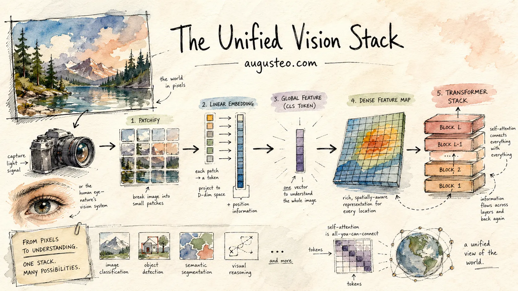
A ViT takes an image (say a 224×224 RGB picture) and chops it into a grid of non-overlapping patches, typically 16×16 pixels each. That’s 14×14 = 196 patches. Each patch is flattened into a vector of pixel values and linearly projected to a fixed-width embedding, say 1024 dimensions. A special “classification token” (an extra learned vector) is prepended to the sequence. So the input to the transformer is a sequence of 197 vectors.

Then: standard transformer layers. Multi-head self-attention followed by feed-forward networks, repeated for dozens of layers. The attention mechanism lets each patch look at every other patch, so by the time we reach the top of the stack, every patch’s vector has been shaped by information from every other patch.

# What a ViT forward pass looks like, roughly
def vit(image):
    patches = chop_into_16x16(image)           # 196 patches of 256 pixels
    tokens  = linear_project(patches)          # 196 vectors of dim 1024
    tokens  = prepend(CLS_TOKEN, tokens)       # now 197 vectors
    tokens  = add_positional_encoding(tokens)
    for layer in transformer_layers:
        tokens = layer(tokens)                 # each token attends to all others
    global_feature = tokens[0]                 # the CLS token
    dense_features = tokens[1:]                # the 196 patch tokens
    return global_feature, dense_features

At the end of the stack, the vector at position 0 (the CLS token) is your global feature. The vectors at positions 1 through 196 are your dense features, each one representing what’s at that patch’s location in the image. The attention mechanism has already mixed information between patches, but each final token is still positionally anchored to its input patch.

This is nice, clean, general. A single architecture that naturally produces both global and dense features. You can scale it by making the tokens wider, the layers deeper, or the patches smaller. The scaling behavior is smooth and well-understood from the NLP side.

And yet.

4. The paradox: scaling made it worse

If you take a ViT and train it on enough data for long enough, something strange happens. The global features keep getting better. Classification accuracy on ImageNet climbs monotonically, breaking past 85%, past 88%, past 90%. The model is clearly learning more and more about images.

The dense features, meanwhile, peak early and then get worse.

This isn’t a subtle effect. Researchers have measured it carefully: on standard dense-feature benchmarks like ADE20k semantic segmentation and Pascal VOC, the quality of a large ViT’s dense features rises during the first few hundred thousand training iterations, peaks, and then degrades steadily until the features become nearly unusable for pixel-level tasks. The phenomenon is called dense feature collapse, and it only really shows up at scale. Smaller models (around ViT-Large, roughly 300M params and below) don’t suffer from it much, because they don’t have the capacity to aggressively specialize toward any one objective and just produce mediocre-but-balanced representations. Past that scale, the model has the capacity to aggressively optimize the loudest signal in the loss function, which, for self-supervised training, is the global clustering objective. The fine-grained per-patch distinctions that dense tasks depend on get sacrificed to make the global summary cleaner.

Why does this happen? The intuition, once you see it, is hard to unsee.

The self-supervised training objective is fundamentally a clustering objective. It asks: “given two views of the same image, make their global summaries land in the same place in embedding space.” In other words, it rewards the model for saying that two patches (a patch of fur from view A and a patch of fur from view B) describe the same thing.

But “describe the same thing” is a slippery requirement. The easiest way to satisfy it is to make all patches of anything-dog-related look similar in feature space. Fur patches, eye patches, ear patches, paw patches: push them all toward a shared “dog” region of the feature space. That’s great for classification, because now a simple average of the patch features is a clean signal for the dog concept. But it’s disastrous for segmentation, because now the model has no way to tell a fur pixel from an eye pixel. They’re in the same neighborhood of feature space.

The longer you train, the more the global objective wins. Patches get pulled toward semantic centers. Local distinctions dissolve. The model becomes a better classifier and a worse mapmaker, and there’s no obvious way to stop the dissolution without also stopping the improvement.

The same loss that teaches the model to see teaches it to stop looking.

This is the paradox that every paper we’re going to discuss is ultimately responding to. The story of modern vision foundation models is the story of a series of increasingly clever ways to preserve local detail while still letting global understanding improve. Three in particular (DINOv3, C-RADIOv4, and FeatSharp) form a coherent stack that now dominates the state of the art.

We’ll take them one at a time.

Act 1 — The Lens

DINOv3, self-supervised learning at scale, and the trick that saved dense features.

5. Meet DINOv3

DINOv3 is Meta’s self-supervised vision transformer, released in August 2025. It is, at the time of writing, the strongest general-purpose vision backbone in the world. It comes in sizes from 21 million parameters (deployable on a laptop) up to 6.7 billion parameters (the research flagship). It was trained on 1.7 billion images without a single human-provided label.

Three things make DINOv3 interesting. First, it took self-supervised learning to a scale nobody thought it could reach: 12× more data and roughly 6× more parameters than its predecessor DINOv2. Second, it produced dense features so good that a frozen DINOv3 backbone outperforms specialized networks on tasks like satellite canopy-height estimation and medical pathology, without any fine-tuning. Third, it solved dense feature collapse (the paradox we just described) with a clean technique called Gram anchoring.

Gram anchoring is the real contribution. Everything else (the scale, the data curation, the architecture tweaks) is table stakes for a 2025 foundation model. Gram anchoring is the idea that will still be influential in five years. Before we can appreciate it, though, we need to understand two pieces of machinery: self-supervised learning, and the Gram matrix itself.

6. Self-supervision, from first principles

If you’re coming from supervised learning, the obvious question is: how do you train a model without labels?

The trick is to invent your own labels by exploiting the structure of the data. In images, a lot of structure is available for free. Two crops of the same image should “mean” the same thing. A masked-out patch of an image should be predictable from the patches around it. A rotated image is still the same image. These are all free sources of supervision. They require no human annotation, just a clever way of asking the model a question whose answer can be checked automatically.

The DINO family (DINO, DINOv2, and now DINOv3) uses a specific technique called self-distillation. Here’s how it works.

You have two copies of the network: a student (which you actively train) and a teacher (which is updated as a slow-moving average of the student’s weights, an exponential moving average, or EMA). Both networks are the same architecture. The teacher is always a slightly stale version of the student.

On each training step, you take a single image and produce two different “views” of it: two random crops, different augmentations, different scales. The student sees one view. The teacher sees the other. Both produce a feature vector. You compute a loss that says: “student, your feature should look like the teacher’s feature.” Then you backprop through the student, and the teacher updates by sliding toward the student’s new weights.

This procedure has no obvious reason to work. There’s no ground truth. The teacher is just another copy of the student, slightly behind in time. You could imagine the whole thing collapsing into a trivial solution: the student outputs a constant vector, the teacher outputs the same constant vector, everyone’s happy and nothing has been learned.

Preventing that collapse is a big part of what the DINO papers are about. The tricks include: careful output-space normalization (via Sinkhorn-Knopp soft clustering), an asymmetric crop scheme (the teacher only sees two large “global” crops of the image; the student sees those global crops plus several smaller “local” crops, and has to match the teacher’s global view from every one of its own views, including the tiny zoomed-in ones), and a lot of temperature-scaling gymnastics. What matters for us is that it does work, and when it works, it works spectacularly. The features DINO learns are so good that frozen DINO backbones (no task-specific fine-tuning) routinely beat specialized supervised networks on individual tasks.

On top of the self-distillation loss (which enforces global consistency), DINOv3 adds a second loss called iBOT, which is a masked patch prediction objective. Some percentage of the patches in the student’s input are masked out (replaced with a special learnable “mask” token) and the student is trained to produce features for those masked patches that match what the teacher would have produced if it had seen them. This is the vision analog of BERT’s masked-language-modeling objective, and it specifically targets local quality: the student has to learn something about each patch that lets it stand in for the real content.

Two losses. One global, one local. Trained together for a million iterations on 1.7 billion images. You might reasonably ask: if iBOT is explicitly a local-quality objective, shouldn’t it prevent dense collapse? The short answer is that at multi-billion-parameter scale, the global DINO pressure (which is what the whole network is fundamentally oriented around) simply outweighs iBOT’s local pressure. iBOT buys some protection early in training. It’s not enough on its own. For the first couple hundred thousand iterations, everything is fine. Somewhere around iteration 200,000, something breaks.

An aside on data. The 1.7-billion-image dataset, called LVD-1689M, was not just scraped off the internet. It was filtered down from a starting pool of about 17 billion web images using an algorithm called hierarchical k-means clustering.

The intuition: the internet is skewed. If you train a model on whatever images happen to be popular on social media, it sees millions of selfies and vacation photos but almost no industrial equipment, medical imagery, or aerial photography. The resulting model learns the skew. Hierarchical k-means groups images into categories, then sub-categories, recursively. Training draws samples uniformly from the leaf clusters rather than from the raw distribution. Rare concepts get proportional attention. Common concepts don’t drown them out.

Think of it as stratified sampling on steroids. You get to see every corner of visual reality, not just the bright-lit center.

7. A Gram matrix, from scratch

To understand DINOv3’s fix for dense feature collapse, we need to introduce one more piece of math: the Gram matrix. It sounds technical but the idea is almost absurdly simple.

Start with a set of vectors. For our purposes, imagine the dense features coming out of a ViT: one vector per image patch. Say we have 196 patches, so 196 vectors, each maybe 1024 dimensions wide.

The Gram matrix of those vectors is a square table where entry (i, j) is the dot product between vector i and vector j. If you have 196 vectors, the Gram matrix is 196 by 196. It doesn’t care about the raw values of the vectors. It only records how they relate to each other.

Let’s do a concrete tiny example. Suppose we have only 4 patches, labeled A, B, C, and D. A and B are both patches of sky. C is a patch of fur. D is a patch of grass. The model produces a 3-dimensional feature vector for each patch:

A few things worth noting about this object. The Gram matrix is square: if you have n vectors it’s n-by-n. It’s symmetric (dot products don’t care about order), so entry (i, j) equals entry (j, i). The diagonal entries are each vector’s similarity to itself, which, if the vectors are normalized to unit length, is always 1.

Here’s the critical property. The Gram matrix doesn’t care about the magnitudes or orientations of the underlying features. If you rotated all your feature vectors by the same angle in feature space, the Gram matrix would be unchanged. If you scaled them all by the same factor, it would change in a uniform, predictable way. What the Gram matrix captures is the relational structure: the geometry of the feature cloud, not its location.

For a vision model, the Gram matrix of the dense features tells you which patches the model thinks are similar and which it thinks are different. If the matrix is “clean” (high values for patches of the same content, low values for patches of different content), the model has a good local map. If the matrix is “noisy” (random-looking similarity everywhere), the model has lost its map.

Dense feature collapse, when you plot the Gram matrix of a late-training ViT, looks exactly like static on an old TV. Every patch looks moderately similar to every other patch. The fine distinctions are gone.

8. Gram anchoring: the blueprint trick

Now we have everything we need to understand Gram anchoring. The DINOv3 team observed the collapse, and they had a specific observation: the Gram matrix used to look fine, earlier in training. At iteration 100-200k or so, the dense features were sharp, the Gram matrix was clean, the model was doing the right thing. The collapse happened later, as the global objective started to dominate.

What if you could hold on to the early, healthy Gram matrix? What if, during late-stage training, you added a new loss term that said “student, your current Gram matrix should stay close to the Gram matrix of your own past self”?

This is Gram anchoring. The details:

1. Take a snapshot of the model at an earlier training checkpoint, chosen while the dense features are still sharp, before collapse has set in. Call this the Gram teacher. Hold it fixed for now. (It will be refreshed periodically, every 10k iterations or so, by copying in the current EMA teacher’s weights. The early-snapshot intuition is what matters; the refresh schedule is a practical detail.)
2. During later training, on each batch, run the image through both the current student and the current Gram teacher. Compute both Gram matrices: G_student and G_teacher.
3. Add a new term to the loss: the Frobenius norm of the difference between the two Gram matrices. Written out, it’s ‖G_S − G_T‖²_F, which is just “sum up the squared differences between corresponding cells.”
4. Train as normal. The student keeps its DINO and iBOT losses, but now also has to keep its Gram matrix from drifting away from the frozen snapshot.

It’s worth pausing on why this works, because the logic is subtle. At first glance, anchoring a newer model to an older version of itself sounds like it would prevent learning. You’re telling the model “be like your dumber self.” Shouldn’t that stop the model from improving?

It doesn’t, and the reason is that Gram anchoring doesn’t constrain the features themselves. It constrains only the relationships between features: the Gram matrix. The underlying feature vectors are free to evolve wildly. They can rotate, they can stretch, they can reshape themselves to capture new concepts. As long as the pairwise dot products stay consistent with the snapshot, the anchoring is satisfied.

Keep the blueprint. Upgrade the materials.

A good analogy: imagine a building. The Gram matrix is the blueprint: which walls are load-bearing, which rooms connect to which, how far the bathroom is from the kitchen. The individual features are the materials: the actual drywall, the carpet, the lighting fixtures. You can swap every piece of drywall for marble, change all the lighting, repaint every wall, and the blueprint is unchanged. The structure remains.

That’s why the technique works. The early-training dense features had good structure. The Gram matrix was clean, distinct patches had low similarity, similar patches had high similarity. By preserving that structure during late training, you let the features themselves keep getting richer and more semantically loaded, while refusing to let them dissolve into an undifferentiated soup.

The result, measured on every dense benchmark that exists, is dramatic. Without Gram anchoring, ADE20k segmentation quality peaks early and then falls by tens of mIoU points over the remainder of training: the classic collapse. With Gram anchoring, it keeps climbing and settles at state-of-the-art levels. This is with the exact same backbone, the same data, the same number of iterations. The only difference is one extra loss term that keeps the spatial blueprint intact.

Gram anchoring is also the reason DINOv3 can be used frozen, with no fine-tuning, on a dizzying array of downstream tasks. Video tracking without ever seeing a video. Satellite canopy-height estimation that beats purpose-built Earth-observation networks. Medical pathology on atypical mitotic figures. The features are so spatially clean that they just transfer. You drop them into a new task, add a small linear head, and the result is often state of the art.

Checkpoint: what you know now.

Vision models produce two kinds of features: a global summary and a per-patch dense map. Both matter. Historically, scaling a self-supervised ViT improved one at the expense of the other.

The failure mode is called dense feature collapse: the pressure to group patches by semantic content ends up dissolving the per-patch distinctions that dense tasks need.

DINOv3 fixes it with Gram anchoring: during late-stage training, use an earlier, still-healthy checkpoint as a Gram teacher, and train the model to keep its current Gram matrix close to that teacher’s. This preserves the structure of the patch features without freezing the features themselves.

DINOv3 is now the single strongest vision backbone in the world. But it has one big limitation: it was trained without text, so it has no idea what any object is called. That’s the next problem.

Act 2 — The Prism

Why three specialist backbones can’t coexist at inference, and how C-RADIOv4 fuses them into one.

9. Three teachers, one student

DINOv3 is the best dense-feature model ever made. It is also, in one specific way, useless: you can’t talk to it. You can’t ask “is there a dog in this picture?” and get a yes-or-no answer, because DINOv3 has never seen the word “dog.” It has no alignment with language at all. It was trained on pure pixels, without captions or labels.

For anything involving natural language (zero-shot classification, text-to-image retrieval, visual question answering, multimodal assistants), you need a different kind of model. The standard is SigLIP2, Google’s 2025 image-text model. Conceptually it sits in the lineage of OpenAI’s CLIP (dual image and text encoders aligned in a shared space), but it’s trained with a different loss: a pairwise sigmoid objective that treats each (image, caption) pair as an independent yes-or-no match. The result is the same kind of shared space. Image features and caption features live in the same embedding space, and you can do a dot product between them to measure how well a caption describes an image.

SigLIP2 is excellent at language alignment. It’s also, in a different specific way, awkward for dense work. The standard high-resolution variant C-RADIOv4 distills from, SigLIP2-g-384, uses patch-16 tokenization at 384 pixels, which gives a 24×24 feature grid. Fine for classification, coarse for anything pixel-precise. SigLIP 2 does include a newer “NaFlex” variant that supports native aspect ratios and variable resolutions, but the fixed-resolution teacher is what’s in play here. And SigLIP2’s features don’t preserve the sharp spatial geometry DINOv3 gives you. They’re semantically rich but spatially mushy.

So: DINOv3 has dense features, no text. SigLIP2 has text, no dense features. Surely we also need high-resolution masking (you know, segment-anything), and that’s a whole other specialist: SAM3, Meta’s November 2025 segmentation model. (A point release, SAM 3.1, landed in March 2026 with tracking speed improvements but no architectural change to the backbone, which is what matters here.) SAM3 will happily take a text prompt and return pixel-precise masks for every instance in an image. But it’s a segmenter, not a general-purpose encoder. It doesn’t give you good global features for classification.

SAM3 and DINOv3 look redundant at first glance. They both produce dense features, so if DINOv3 is already excellent at dense work, why do we need SAM3 as a separate teacher? Because the two models come from completely different supervision regimes, and each regime teaches something the other one structurally can’t. DINOv3 is self-supervised: it never sees a label, and certainly never sees a mask. Its loss is a clustering objective that pushes patches of similar content toward the same region of feature space. That’s great for semantic grouping, but it’s blind to where one instance of a class ends and another begins, because the loss has no ground truth for instance identity. Two cars parked next to each other sit in the same region of DINOv3’s feature space, by design.

SAM3 was trained on pixel-exact mask supervision at scale, roughly 4 million unique concepts from Meta’s SA-Co data engine (with instance masks, hard negatives, and both image and video annotations). Every training example carries explicit information about where a specific instance stops, which is information self-supervision cannot produce no matter how much data you scale to. SAM3’s architecture is built around this: its DETR-based detector has a dedicated presence head that separates “is this concept in the image” from “where exactly is each copy of it.” The backbone (Meta’s Perception Encoder) is pre-trained separately and then coupled to the detector, with a later tracker stage that runs on top of a frozen backbone.

This matters for C-RADIOv4 in two ways. First, the student’s dense features inherit information that’s structurally absent from the DINOv3 signal: instance-level discriminability, and features shaped by a pixel-exact boundary loss. Second, because the student is distilled specifically to match the Perception Encoder’s output format, C-RADIOv4 can function as a drop-in replacement for SAM3’s backbone. Swap it in, keep SAM3’s detector and tracker unchanged, and you get the whole promptable-segmentation and video-tracking stack at a fraction of the encoder cost. That kind of compatibility is at least part of the appeal of SAM3 as a teacher.

Three backbones. Three complementary strengths. And running all three in production is expensive enough that most teams won’t do it. A ViT-H at 1024 pixels isn’t cheap on its own; running two or three of them in parallel multiplies your inference cost for every request, and multi-encoder VLM stacks are the kind of thing you build reluctantly rather than by design. Getting the same capabilities out of one backbone is worth real money.

This is where C-RADIOv4 enters the story.

10. What distillation is, really

Before we can talk about C-RADIOv4, one more piece of background. The technique C-RADIOv4 relies on is called knowledge distillation, and it deserves a careful explanation because the whole story turns on it.

The simplest version of distillation was introduced by Geoffrey Hinton in 2015. You have a big, slow model (the teacher) that’s been trained on some task. You want a small, fast model (the student) that does the same task almost as well. Training the small model from scratch on the original labels gives you mediocre results. But if you use the teacher’s outputs as soft targets for the student, the student does dramatically better than it would if it were just mimicking the ground-truth labels.

The reason is that the teacher’s outputs contain more information than the labels do. A label is a single correct answer. A teacher’s output is a probability distribution over all possible answers, which encodes relationships: “this looks 80% like a cat, 15% like a lynx, 5% like a fox, nothing else.” The student learns the teacher’s full landscape of what’s similar to what, not only the right answer.

Now: what if, instead of distilling from one teacher, we distill from several? What if we have a set of specialist teachers, each expert at a different aspect of vision, and we train a student whose job is to match all of their outputs simultaneously?

This is multi-teacher distillation, and it’s the core idea behind the RADIO family of models (of which C-RADIOv4 is the latest). The student doesn’t try to recreate any single teacher. It learns a unified embedding (a single feature vector) from which all the teachers’ output features can be predicted. Small heads on top of the student are trained to reproduce DINOv3’s output, SigLIP2’s output, and SAM3’s output, respectively. But the backbone itself is shared.

Crucially, this is an agglomerative process: the student ends up carrying information from all three teachers, because it has to serve all three of their prediction heads. At inference time, you run the student once (one forward pass) and you get features that can be used for any of the downstream tasks. If you need DINOv3-style dense geometry, read off the dense features. If you need SigLIP2-style text alignment, pass through the SigLIP2 head. If you need SAM3-style segmentation, pass through the SAM3 head. The expensive forward pass happens once. The lightweight heads run in microseconds.

This all sounds elegant and easy. In practice, naive multi-teacher distillation with teachers that have very different activation statistics runs into a known failure mode: the student disproportionately learns the teacher with the loudest loss and underfits the quieter ones. The PHI-S paper documents this quantitatively. Text alignment capabilities are the typical casualty when DINO-style teachers are in the mix, because their feature distributions are much wider.

The reason, it turned out, was geometry.

11. Why three teachers clash

Let’s go back to feature space. Imagine DINOv3’s output features as a cloud of points in a high-dimensional space. Each image produces one point. The cloud as a whole occupies some region of the space. How big is that region? How spread out are the points?

This property (how widely a set of feature vectors spreads out in its space) has a technical name: angular dispersion. You can measure it empirically by taking a large batch of images, encoding each one, and computing the average angle between every pair of features. A cloud that’s tightly clustered has low angular dispersion. A cloud that fans out widely has high angular dispersion.

Here are the measured values, from the C-RADIOv4 paper:

• DINOv3-7B — dispersion ≈ 2.186
• SigLIP2-g — dispersion ≈ 0.694

DINOv3’s features spread over roughly three times as much angular volume as SigLIP2’s. The geometric analogy: DINOv3 is a floodlight, casting a broad cone. SigLIP2 is a laser pointer, emitting a narrow beam.

Why does this kill naive distillation? Because of how distillation losses work. The student is trained to match each teacher’s output. The loss for each teacher is something like “squared distance between student’s prediction and teacher’s target,” averaged across a batch.

If DINOv3’s features are spread over a wide angular range, the typical distance from one DINOv3 feature to another is large. Large distances mean large loss values. So DINOv3’s loss contribution to the total loss (summed across all teachers) is large. SigLIP2’s features are bunched tightly together, so their distances are small, so their loss contribution is small.

When you backpropagate, gradient magnitudes scale with loss magnitudes. DINOv3’s gradient dominates. SigLIP2’s gradient gets drowned out. The student optimizes the thing that’s loudest, which is DINOv3, and ignores the thing that’s quiet, which is SigLIP2. End result: you’ve trained a DINOv3 lookalike with a vestigial, useless SigLIP2 head.

This is a geometric problem, and it has a geometric solution.

12. Three ingredients of the C-RADIO recipe

The C-RADIOv4 tech report builds on a set of tricks that have been accumulating in the RADIO line for a while. Two of them — PHI-S and shift equivariance — were introduced in earlier RADIO papers (2024) and refined in v4. The third, stochastic multi-resolution training, is the natural culmination of work on the “mode switching” problem that has been chipped away at across several releases. Taken together, they’re the core ingredients that make agglomerative distillation work at all.

Ingredient 1: Balanced Summary Loss (PHI-S)

Divide each teacher’s loss contribution by that teacher’s angular dispersion. Before the losses get summed, DINOv3’s loss gets scaled down by 2.186 and SigLIP2’s loss gets scaled up (or equivalently, scaled down by 0.694). After this normalization, both teachers contribute the same total gradient magnitude. The floodlight and the laser pull with equal force.

The exact technique, which NVIDIA calls PHI-S (for “PHI-Standardization”), goes a bit further than dividing by a single dispersion number. Under the hood it applies a Hadamard rotation to each teacher’s feature space and then standardizes the resulting dimensions uniformly, so that the distribution becomes isotropic: no direction in the feature space dominates any other. The practical effect is the one you’d expect — the student is forced to learn the shape of each teacher’s feature space, not just its loudest directions — and the “divide by dispersion” framing above captures the spirit even if the mechanics are a little fancier. (Note: PHI-S was introduced earlier in the RADIO line, around v2.5 in 2024. C-RADIOv4 inherits it rather than introducing it.)

After PHI-S, multi-teacher distillation actually works. The student carries all three teachers’ capabilities in a single embedding. But we’re not done. There are still two subtle failure modes that show up when you try to distill from many teachers at once.

Ingredient 2: Shift Equivariance

Here’s a problem nobody thinks about until they’re deep into multi-teacher distillation: every teacher has bad habits. Little position-dependent quirks that aren’t really about the image content but are artifacts of how the teacher was trained.

A famous example in the ViT literature: large self-supervised models tend to produce a handful of “artifact tokens”: patches with anomalously large activations that don’t correspond to anything in the image but instead get used as scratchpad memory for the network. DINOv3 actually addresses this with an architectural trick called register tokens: four extra learnable tokens prepended to the sequence, specifically designed to absorb the scratchpad role so that the real patch tokens can stay clean. That helps a lot. But it doesn’t eliminate every position-locked quirk. Residual patterns survive in all the teachers. SigLIP2 has dead zones along the borders of its feature maps, because its training data was cropped and the border regions saw systematically less variation. SAM3 has grid-aligned artifacts that come from its windowed attention pattern. DINOv3 still has subtler traces tied to specific coordinates in its positional encoding.

None of these habits are properties of the input image. They’re properties of the teacher’s architecture and training, anchored to specific pixel coordinates. When you distill naively, the student learns these artifacts faithfully and bakes them into its own features forever.

The fix: shift equivariance. During training, take the student’s input and translate it by a random small offset. Shift the image left by 7 pixels, say. The teacher sees the original un-shifted image. When you compare student and teacher outputs, you un-shift the student’s feature map (moving it back to align with the teacher’s) before computing the loss.

Now think about what these artifacts have in common. The border dead zones are at fixed pixel coordinates. The SAM3 grid artifacts are at fixed pixel coordinates. Any residual position-locked pattern lives at fixed pixel coordinates. In the un-shifted student’s feature map, the “corresponding” patch is at a different pixel coordinate every batch, because the shift offset changes randomly. So the artifacts stop correlating with anything. The student can’t learn to produce them, because there’s no fixed position where they consistently appear. The student gives up memorizing positions and learns only the input-content-dependent part of each teacher’s signal.

It’s a minimal fix. One line of code during training, and an entire class of inherited garbage disappears from the student’s features.

Ingredient 3: Stochastic Multi-Resolution

The third ingredient concerns a subtle issue you only notice when you try to use a model at many different resolutions. Standard ViT training happens at a single fixed resolution, usually 224px or 336px. When you deploy the model and someone sends it a 1024px image, you’re asking it to generalize to a regime it never saw.

What ends up happening, in practice, is the model learns two modes. One mode works at the training resolution and assumes certain statistical properties of the input (fixed number of patches, fixed receptive field, fixed position indices). Another mode, activated when the image is much larger, has to awkwardly interpolate. The two modes conflict. The same features don’t mean the same thing at 224px and 1024px. Inference becomes brittle. Downstream tasks that need a specific resolution work great; tasks that need a different one suddenly fail.

C-RADIOv4 solves this by randomly sampling the training resolution on every batch, from a discrete set that spans low resolutions (128, 192, 224, 256, 384, 432) and high resolutions (512, 768, 1024, 1152). The student learns a single representation function that works at every scale. No modes. No special cases. One checkpoint serves any resolution at inference.

This also has a lovely side effect: it lets C-RADIOv4 track the full scaling curve of DINOv3-7B at a fraction of the parameter count. A 631M-parameter C-RADIOv4-H student matches (and often exceeds) an 840M-parameter DINOv3-H+ on dense benchmarks, precisely because the student has been pressured by multiple teachers to be efficient. It can’t afford to waste parameters on resolution-specific specializations.

Checkpoint: what you know now.

No single vision backbone does everything well. DINOv3 has dense self-supervised features but no text and no instance separation. SigLIP2 has text alignment but no dense spatial structure. SAM3 has mask-supervised features with instance separation but narrow global semantics.

Multi-teacher distillation can fuse them into one student, with three key ingredients accumulated across RADIO releases:

(a) PHI-S normalization so that the floodlight and the laser contribute equal gradient weight; (b) shift equivariance so the student doesn’t inherit position-locked teacher artifacts; (c) stochastic multi-resolution so the student learns a single scale-invariant function instead of a per-resolution mode.

The result is C-RADIOv4: one backbone that runs all three teachers’ capabilities in a single forward pass, with 412M or 631M parameters depending on the variant.

But we have one problem left. The trick only works if all three teachers can produce usable targets at the training resolution. DINOv3 can. SAM3 can. SigLIP2 cannot.

Act 3 — The Dial

FeatSharp, a 2D upsampler built on a 3D reconstruction trick.

13. Resolution, the last mile

SigLIP2 was trained at 384×384. Its feature map, at that input resolution, is 24×24, one vector per 16×16 pixel patch. If you ask SigLIP2 to process a 1152×1152 image, its internal machinery gets cranky. Position embeddings, which were learned at the training resolution, now have to extrapolate. The feature map becomes 72×72, but the patches at those new positions have position encodings the model has never seen. The features degrade, not catastrophically, but visibly. Boundaries become fuzzy. Patterns repeat where they shouldn’t. Textures look like plaid.

You can see it with your eyes if you run a PCA on the feature map and visualize it as a color image. At 384px, SigLIP2’s features look clean, crisp, object-aware. At 1152px via simple bilinear interpolation, they look like a defocused photograph.

The problem for C-RADIOv4: if the training resolution is random between 128px and 1152px, the student sometimes sees images at 1152px. At that resolution, the student needs to produce features that match SigLIP2’s features. But SigLIP2 can’t produce clean features at 1152px. The supervision signal is noise. The student learns nothing useful from SigLIP2 at high resolutions, which means its text-alignment capabilities stay weak.

We need a way to get clean SigLIP2 features at 1152px, without retraining SigLIP2. This is the job of FeatSharp.

14. The NeRF trick for features

To explain FeatSharp, I have to briefly talk about NeRF. NeRF (Neural Radiance Fields) is a 3D reconstruction technique from 2020. Its setup is this: you have a few dozen 2D photographs of a real-world scene, taken from different viewpoints. You want to reconstruct a 3D representation of the scene that you can render from any new viewpoint.

NeRF’s core insight is a consistency principle. A real 3D point in the scene is observed in multiple 2D photos. When you look at where that point projects to in photo A, you see a specific color. When you look at where it projects to in photo B (from a different angle), you see that same color, or something close to it, depending on lighting. Features of real 3D structure are consistent across views.

Conversely: anything that varies across views is not real 3D structure. It’s an artifact: sensor noise, specular reflection, glare, occlusion, something that isn’t part of the stable underlying scene.

NeRF uses this to build a coherent 3D representation: it finds the 3D structure that, when rendered to the 2D photographs, is consistent with all of them. Parts that can’t be made consistent are rejected as noise.

Now: the same principle applies, in a totally different setting, to feature upsampling.

Imagine you have a low-resolution encoder, say SigLIP2 at 384px. You want its feature map at 1152px. Naive bilinear interpolation will hallucinate details the encoder never committed to. But what if you exploit consistency across views of the feature map?

Here’s the FeatSharp recipe:

1. Take the input image. Jitter it slightly: shift it by a few pixels, crop it differently, flip it horizontally, mess with its alignment. Generate many small variations (“views”) of the same underlying scene.
2. Run the low-resolution encoder on every jittered view. Collect the feature maps. They’re all low-resolution, but they’re all slightly misaligned versions of roughly the same content.
3. Learn a high-resolution feature map such that, when you apply the corresponding jitter and downsample to low resolution, the result matches each view’s low-res feature map.
4. Features that are consistent across views of the same content survive the upsampling process. Features that flicker, changing from one jitter to the next, get suppressed.

The result: a clean, high-resolution SigLIP2 feature map that is fully consistent with what SigLIP2 would have produced at low resolution, and contains only the details that survive the multi-view consistency test. No hallucinated boundaries. No plaid artifacts. A supervision signal C-RADIOv4 can actually learn from.

FeatSharp is a small module, about as expensive as one extra transformer block, and it plugs into the C-RADIOv4 training pipeline as a preprocessor for SigLIP2’s targets. It’s also useful independently: any time you have a pretrained low-resolution vision encoder and want to extract richer spatial information from it, FeatSharp can upgrade the feature resolution without retraining the encoder.

15. Interlude: borrowing from biology

Before we put the whole pipeline together, one more idea deserves its own section. It’s used across all three papers we’ve discussed, but it’s not really about computer vision. It’s about how neural networks should be trained in the first place. And it’s borrowed, more literally than is typical, from biology.

Here’s the setup. When you train a neural network, a common trick for improving robustness is to inject noise somewhere in the training process. Add a bit of Gaussian noise to the inputs. Add dropout to the activations. Add weight decay to the gradients. All of these are additive perturbations, and they all work reasonably well.

Biological synapses work differently. Real synapses in real brains do something called multiplicative noise. The fluctuation in a synaptic signal is proportional to the signal’s magnitude. When a synapse is firing weakly, its noise is small. When it’s firing strongly, its noise is big. The ratio stays roughly constant, a 10% jitter around whatever the signal is. This follows a log-normal distribution, which has been measured experimentally in mouse brains, rat brains, human brains. It’s a universal property of biological neural machinery.

Another way to see the difference: imagine the volume knob on a stereo. If the music is playing quietly and you bump the knob slightly, you barely notice. If the music is already at maximum volume and you bump the knob by the same amount, the change is enormous and chaotic. Biological noise is the second kind. Additive noise in standard ML training is the first kind. They produce qualitatively different optimization dynamics.

In 2024, a paper called DAMP (Data Augmentation via Multiplicative Perturbations) made a clever observation: an input corruption, to first order, looks a lot like a multiplicative perturbation of the weights in the downstream layer. So instead of augmenting the data, you can augment the weights: multiply each weight by a small random Gaussian during the forward pass, and train normally. DAMP demonstrated that this is enough to produce networks that are dramatically more robust to real-world input corruptions. No extra data, no extra forward passes. Just change the noise structure.

DAMP’s justification is geometric, not biological. But the family of techniques it opens up turns out to line up closely with what biology does. In 2025, LMD (Log-Normal Multiplicative Dynamics) made the biological motivation explicit: it derives a Bayesian learning rule that assumes log-normal posterior distributions over weights, directly inspired by the log-normal distribution of biological synaptic weights, and uses multiplicative updates with both noise and regularization applied multiplicatively. LMD achieves stable training at very low numerical precision, which matters a lot for next-generation hardware.

C-RADIOv4’s training recipe explicitly uses both DAMP and a related technique, MESA (Memory-Efficient Sharpness-Aware Training), a cousin of these methods that approximates Sharpness-Aware Minimization via a trajectory loss against an EMA teacher, driving the optimizer into “flat” regions of the loss landscape, where small perturbations don’t change the loss much. Flat regions generalize better than sharp regions. So you get the same dataset, the same architecture, and a model that degrades more gracefully on unseen data. Closely related in spirit: ASAM (Adaptive SAM) has been shown to be mathematically equivalent to optimizing under adversarial multiplicative weight perturbations, which is what ties the sharpness-aware line back to the multiplicative-noise story in this section.

The bigger lesson: a lot of ML practice inherits assumptions from statistics textbooks (Gaussian noise, L2 penalties, isotropic distributions) that have nothing to do with how biological computation actually works. Occasionally, questioning those assumptions and reaching into neuroscience produces a free lunch. Multiplicative weight perturbation is one of the cleanest free lunches of the last few years.

There’s a philosophical angle worth noting. We’ve spent two decades assuming that biological intelligence and artificial intelligence are “different kinds of systems,” and that trying to directly translate neural biology into deep learning is a mug’s game. Sometimes that’s right. Backpropagation is not how brains learn, and anyone who says otherwise is selling something. But the log-normal synapse story is a counterexample. A specific, measured, boring property of real neurons (their noise is proportional to their signal) turns out to make artificial networks measurably better when imitated. Not every biological property will. Some of them will. The field is slowly learning which.

16. Putting it together: the pipeline

Let’s zoom back out. We’ve now covered every piece. Here’s the full training pipeline for a 2026 vision foundation model, from raw images to deployable checkpoint.

There’s one more piece worth explaining: how the pipeline scales down for deployment. The 6.7-billion-parameter DINOv3-7B model is wonderful for research, terrible for production. It’s slow, expensive, and hard to serve. Most real use cases want a model that fits on a single GPU, runs in under 100ms, and doesn’t require a dedicated inference cluster.

The solution is multi-student distillation. Instead of training one small student to mimic the big teacher, you train an entire family of them simultaneously: a ViT-Small (21M params), a ViT-Base (86M), a ViT-Large (304M), a few ConvNeXt variants, all at once. The real trick: you only run the expensive teacher once per batch. Cache its outputs. Then broadcast those cached targets to every student. Each student consumes the same distillation signal but learns its own efficient architecture.

This is how a 6.7B self-supervised teacher ends up producing a 21M ConvNeXt you can put on a Jetson. It’s also why the DINOv3 “model family” includes so many sizes: Meta trained them all in parallel, sharing the teacher’s compute across every student.

Checkpoint: what you know now.

The full pipeline: pretrain a big ViT with self-supervision → repair dense features with Gram anchoring → adapt to arbitrary resolutions → distill multiple specialist teachers into a unified student → distill the student into many smaller students for deployment.

The output: a family of vision backbones ranging from 21M to 840M parameters (and a 6.7B research flagship on the DINOv3 side) that all share the same fundamental capabilities (classification, segmentation, depth estimation, text alignment, video tracking, cross-domain transfer) in a single forward pass. You pick the size that fits your hardware budget.

17. Three ideas worth stealing

We’ve covered a lot of ground: self-supervision, Gram matrices, multi-teacher distillation, angular dispersion, NeRF-inspired upsampling, log-normal synapses. If you only take three things away from all of it, I would pick these:

1. Regularize relationships, not values.

Gram anchoring is the cleanest example of a pattern that keeps showing up across machine learning: when some property of your model is degrading during training, the fix is often not to freeze the values of the relevant quantities but to freeze their relational structure. The Gram matrix preserves pairwise similarities while letting individual features evolve. The underlying idea, pin the geometry and free the content, is applicable far outside vision. Any time you have a representation that you want to stay structurally coherent while continuing to learn new things, ask what relational property captures the structure you care about, and regularize that.

2. Heterogeneous signals need geometric normalization.

The C-RADIOv4 three-teacher problem is, at its heart, a generic issue with combining evidence from sources with different natural scales. Naive weighted averaging fails silently when the sources have different variances or different angular ranges. You don’t get a helpful error message; you get a model that ignored the quieter source. The fix is to normalize by each source’s intrinsic scale before combining. PHI-S is one specific way to do this in feature space, but the general principle (measure each source’s natural magnitude and divide it out before summing) applies broadly. Multi-loss optimization, multi-task learning, sensor fusion, ensemble methods: all of them have this failure mode, and the fix is always some variant of the same normalization.

3. Randomize what you don’t want memorized.

Shift equivariance, stochastic multi-resolution, multiplicative weight perturbation: these are all, at some level, the same trick. If there’s a structural property of your training setup that you don’t want the model to encode as a shortcut, randomize it during training. Fixed pixel coordinates become random offsets. Fixed resolutions become sampled resolutions. Fixed noise levels become proportional fluctuations. The model learns the part that’s invariant to the randomization, which, by construction, is the part you actually want it to learn. This is an old idea dressed up in many clothes, but it bears repeating: if your model is learning something you didn’t intend, look for a way to make that something vary from batch to batch, and watch it disappear.

Epilogue

It’s tempting to read the story of DINOv3 / C-RADIOv4 / FeatSharp as a procession of clever technical tricks, each patching over a specific failure mode. That’s true, but it’s not the whole truth. What’s really happening, I think, is that the field is converging on a more mature understanding of what a vision model is.

The early ViT models were trained on one objective and evaluated on one benchmark. They were good at that benchmark and bad at everything else. The 2025–2026 generation is trained on multiple objectives, evaluated on dozens of benchmarks across domains the model was never specialized for, and expected to do all of it from a single frozen backbone. The architecture didn’t really change. What changed is the training recipe and, more importantly, the understanding of what constraints the recipe needs to satisfy for the resulting features to be useful in the wild.

Gram anchoring is a constraint. Shift equivariance is a constraint. Multi-resolution sampling is a constraint. Multiplicative noise is a constraint. Each one narrows the space of functions the model can learn, in exchange for making the functions that remain more robust, more transferable, more general. The field is learning to write down the right constraints.

If there’s a pattern here beyond computer vision, it’s this: modern machine learning is increasingly about finding the right structure to preserve, not the right thing to learn from scratch. Gradient descent will learn almost anything, given enough data and compute. Making it learn the right thing (the thing that transfers, the thing that generalizes, the thing that survives contact with reality) is a matter of writing down what must remain invariant. Dense feature structure must remain invariant to continued training. Cross-teacher gradients must remain balanced. Feature maps must remain invariant to small input shifts. Performance must remain invariant to resolution. These are not subtle philosophical demands. They are engineering constraints, with concrete losses and concrete training tricks that enforce them.

The payoff is real. A single DINOv3 backbone beats specialized Earth-observation networks at satellite tree-height estimation. A single C-RADIOv4 backbone, at 631 million parameters, ties or beats its much larger peers (including DINOv3-H+, an 840M distilled sibling of its 7B teacher) on dense benchmarks. A single inference call provides classification, segmentation, depth, tracking, correspondence, text alignment, and open-vocabulary masking. The vision backbone is becoming, increasingly, just a backbone: a single spinal cord that a thousand downstream heads can read from.

Which is, when you think about it, pretty close to how biological vision works. A single visual cortex produces a representation that the rest of the brain interprets in a dozen different ways, for a dozen different purposes, using a dozen different downstream circuits. The representation is fixed; the interpretations are flexible. It took artificial vision a while to get there. It seems to be arriving.

We used to think the blurry mess was a failure of the machine. It turns out the blur was a failure of the objective.

References

• DINOv3. Siméoni et al., Meta AI 2025 (arXiv:2508.10104).
• C-RADIOv4 Tech Report. Ranzinger et al., NVIDIA 2026 (arXiv:2601.17237).
• FeatSharp. Ranzinger et al., NVIDIA 2025 (arXiv:2502.16025).
• PHI-S (distribution balancing). Ranzinger et al., NVIDIA 2024 (arXiv:2410.01680).
• DAMP (multiplicative weight perturbations). Trinh et al. 2024 (arXiv:2406.16540).
• LMD (log-normal multiplicative dynamics). Nishida et al., RIKEN AIP 2025 (arXiv:2506.17768).
• SAM 3. Meta AI 2025 (arXiv:2511.16719).
• SigLIP 2. Tschannen et al., Google 2025.

Originally prepared for the Boon engineering team, April 2026.