The Unified Multimodal Stack

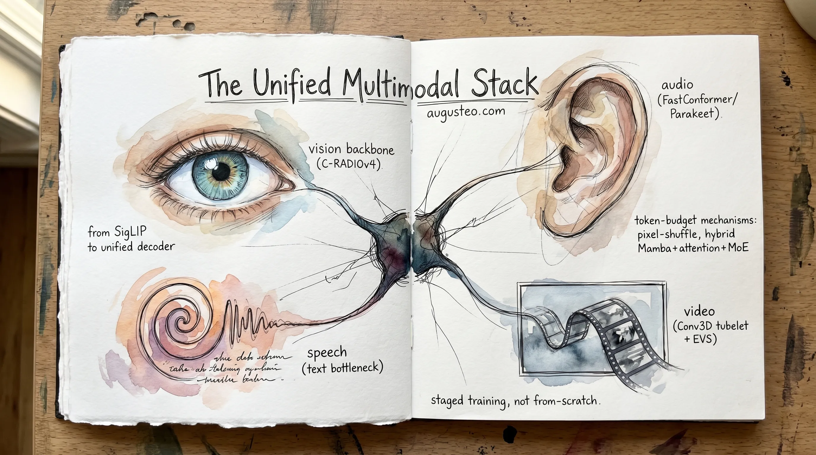
A sequel to The Unified Vision Stack. Picks up where C-RADIOv4 ended and asks what it takes to teach one eye to listen, watch, and speak. Worked example throughout: NVIDIA’s Nemotron 3 Nano Omni, released April 2026. About a 45-minute read.

1. A single eye, three teachers

The previous post left us with C-RADIOv4. One vision backbone, three teachers, a single forward pass whose features could be read by three different downstream tasks at once.

The prequel post walks through C-RADIOv4 in detail: DINOv3 brought dense patch geometry, SigLIP2 brought text alignment, SAM3 brought instance masks, and C-RADIOv4 inherited the three through AM-RADIO-style agglomerative distillation. At inference you can attach a small head to the shared backbone and read off whichever family of feature a downstream task wants.

For this post the relevant takeaway is narrower: the backbone is a strong “vision-only” model. Hand it an image and you can do dense prediction, retrieval, or segmentation through the appropriate head. Other vision tasks the family is reported to handle (depth, tracking, and beyond) are covered in the prequel; here we only need that the backbone can serve as a feature extractor for an LLM.

But “look at an image” is not the job most modern systems are being built for. The thing people want is an agent: something that takes a photo, listens to a question, watches a video, and answers in language. The system has to perceive across modalities and then talk about what it perceived. C-RADIOv4 only handles half of that loop, and only for one of the modalities.

What does the rest take?

There’s a clue in C-RADIOv4 itself. One of its teachers was SigLIP2, so the SigLIP-aligned head on the backbone is trained to put image features into a space shared with text embeddings. SigLIP itself trains image and caption towers to score together (more on the loss in §3); inheriting that head means the C-RADIOv4 backbone can produce vectors that are aligned with caption-space text in the SigLIP sense. We already have, through that head, an image encoder that “speaks text” in that specific sense.

So why does Nemotron 3 Nano Omni, the open omni model NVIDIA shipped in April 2026, still bolt a separate text tokenizer onto the front of a 30-billion-parameter autoregressive language model and feed C-RADIOv4-H’s features into it as if they were just another input? If the SigLIP head was meant to be the text bridge, what does the LLM do that the head can’t?

The short answer is that SigLIP-style alignment scores; it doesn’t generate. Once that’s clear, the rest of the architecture falls into place. The post unfolds three architectural moves: a text-centric autoregressive decoder at the center, modality-specific encoders for everything that isn’t text, and a stack of token-budget mechanisms to keep inference cost from collapsing under its own weight.

Act 1: the puzzle

Why a vision backbone that already aligns to text still cannot answer in language.

2. The SigLIP puzzle

The SigLIP head sitting on top of C-RADIOv4 produces caption-aligned features. An image goes in, a vector comes out, and that vector lives in the same embedding space SigLIP’s text tower lives in. So you can take any sentence, embed it through the text tower, and ask: how close is its embedding to the image’s? You get a similarity score. Higher score, the caption fits the image better. Lower score, it doesn’t.

What you can’t do with that score is ask for a description of the image. The SigLIP text tower never learned to produce sentences. It only learned to score them.

This is easy to lose track of, because SigLIP and CLIP are routinely described as “vision-language models” in a way that suggests they understand language in some general sense. They don’t, in the sense the rest of the post is going to need. Here’s what they actually do, taken straight from the CLIP paper:

“The text sequence is bracketed with [SOS] and [EOS] tokens and the activations of the highest layer of the transformer at the [EOS] token are treated as the feature representation of the text which is layer normalized and then linearly projected into the multi-modal embedding space.”

The text tower runs through the sentence once, takes one vector from one position in the final layer, and stops. Whatever happened in the per-token states gets thrown away. The output is a single embedding that says “this sentence as a whole means X” in some compressed form, and that is the entire output. The training loss never asked the model to expose a per-token next-token distribution, so it never learned to produce one.

SigLIP and SigLIP 2 keep the same shape, just with different losses (sigmoid binary classification per pair instead of softmax over the batch). SigLIP 2 even attaches a decoder during training to push the encoder representations harder, but the decoder gets thrown away before release:

“Finally, we note that the decoder only serves for representation learning here and is not part of the model release.”

So the artifact you actually get is still a contrastive embedder. It scores. If you want to generate, you need a different organ.

The architectural consequence is the central design choice of every modern omni-modal stack. The text decoder sits in the middle. Vision goes in as features. Audio goes in as features. Video goes in as features. The decoder is the only thing in the system that can run a softmax over the next word, and everything else feeds it.

C-RADIOv4 is one of the best things you can put in front of a decoder. It is not, by itself, a decoder.

3. Contrastive vs autoregressive

The split between scoring and generating is structural, not a difference of degree. To see why, look at what each model is being trained to optimize.

CLIP’s loss is the cleanest version. Take a batch of N image-caption pairs. Run each image through the image tower, each caption through the text tower. You now have N image vectors and N text vectors. Compute every pairwise dot product: that gives you an N×N matrix of similarities. The training loss says, for each row of this matrix, the diagonal entry should be the largest (because the image at row i pairs with the caption at column i, the matched pair). For each column, same thing. Apply softmax cross-entropy over the rows and over the columns, average them. That’s the whole loss.

“Given a batch of N (image, text) pairs, CLIP is trained to predict which of the N × N possible (image, text) pairings across a batch actually occurred. … We optimize a symmetric cross entropy loss over these similarity scores.”

SigLIP swaps the softmax for a sigmoid binary classification on each cell of the matrix: each pair is either matched (label +1) or unmatched (label −1), and every cell contributes independently. Computationally cheaper to scale. Same architectural shape: dual towers, dot product, scalar score per pair.

What this loss does not teach the model is anything about next words. The matched-pair signal at any cell tells the towers “make these two embeddings closer.” It says nothing about what should come after a given word in a sentence. Both towers, image and text, are trained to produce one embedding each, then compared. The text tower never has to predict the next token. There is no decoder loss. There is no autoregressive supervision anywhere in the training procedure.

A language model is doing the opposite thing. Take a sentence. For each prefix of the sentence (the first 1 word, the first 2 words, and so on), compute a probability distribution over what the next word should be. The loss is the negative log-likelihood of the actual next word, summed over all positions. This does teach the model about next words. It teaches almost only about next words. After enough data, you have a function that takes a partial sentence and returns a probability distribution over every possible continuation, which you can sample from to make new text.

These are two different functions, and the difference doesn’t shrink with scale. The contrastive function takes (image, sentence) and returns a number. The autoregressive function takes (partial sentence) and returns a probability distribution over the next token. You can’t use one to do the other’s job, no matter how large you make it. Scaling SigLIP doesn’t get you generation. Scaling an LLM doesn’t, by itself, get you a calibrated image-caption similarity score; you have to fit a head on top to extract one.

This is why most production multimodal stacks ship both. SigLIP-class encoders for understanding what’s in an image. An autoregressive LLM in the middle for producing language. (Some research designs go the other way, with an early-fusion model that tokenizes images straight into the LLM’s vocabulary; Chameleon is the cleanest example of that branch. The pretraining cost story for that approach is much larger, and it isn’t the path Nemotron 3 Nano Omni took.)

4. The text decoder is a different organ

The five things an autoregressive LLM contains, in the order an input flows through them: a tokenizer that splits text into sub-word pieces from a fixed vocabulary; a learned embedding table that maps token IDs to continuous vectors; a stack of attention (and sometimes state-space) blocks that produce contextualized hidden states; a learned LM head that projects each hidden state back to the vocabulary as logits; and an autoregressive sampling loop that picks one token from the final logits, appends it to the input, and runs the whole thing again.

Pieces 4 and 5 do not exist in SigLIP’s text tower. SigLIP has the first two (tokenizer, embedding table) and something like the third (a small transformer over the tokens), but the output gets projected once into the shared image-text space and then the model stops. There is no head that produces a distribution over next tokens, and no sampling loop to consume one. The contrastive training objective specifically did not select for them.

So we need an LLM in the middle. The question becomes how to get the vision encoder’s output into the LLM’s input, and the parallel question for audio and video.

Act 2: three ways to wire it up

Once you know you need a generative LLM, the question is how you feed it.

5. The adapter zoo: Flamingo, BLIP-2, LLaVA

Suppose you have a strong text-only LLM. Pretraining cost millions of dollars and you don’t want to redo it. You also have a strong vision encoder, frozen, that produces dense feature maps. The question is: how do you bolt them together so the LLM can answer questions about images without losing what it already knows about language?

Three approaches dominated the 2022-2024 era, and the differences between them turn out to be load-bearing for what came after.

Flamingo (DeepMind, 2022) inserts new layers into the frozen LLM. Specifically, between every pretrained block, Flamingo adds a GATED XATTN-DENSE block: a cross-attention layer where the query is the LLM’s current hidden state and the key/value are visual features (after passing through a Perceiver Resampler that compresses the variable-size feature grid into 64 fixed slots). The cross-attention output is gated by a learned scalar α, multiplied through tanh(α) where α is initialized to zero. At step 0, every new block is a no-op:

“We freeze the pretrained LM blocks, and insert gated cross-attention dense blocks between the original layers, trained from scratch. To ensure that at initialization, the conditioned model yields the same results as the original language model, we use a tanh-gating mechanism.”

The training process pushes α off zero only as the cross-attention starts contributing useful signal. The LLM weights themselves are never updated. Catastrophic forgetting is averted by construction.

BLIP-2 (Salesforce, 2023) takes a different shape. Instead of adding cross-attention into the LLM, it adds a separate small module (a 188-million-parameter Querying Transformer, or Q-Former) between the frozen vision encoder and the frozen LLM. Q-Former has a fixed set of learned “query” embeddings that attend to the vision encoder’s outputs through cross-attention. The output is a short fixed-length sequence (32 vectors in the released checkpoints) that gets linearly projected and prepended to the LLM’s prompt as if it were ordinary text tokens. Q-Former is trained in two stages: first in isolation against an image-text alignment objective, then together with the frozen LLM against a generation loss.

“BLIP-2 bridges the modality gap with a lightweight Querying Transformer, which is pre-trained in two stages. The first stage bootstraps vision-language representation learning from a frozen image encoder. The second stage bootstraps vision-to-language generative learning from a frozen language model.”

LLaVA (Microsoft and Wisconsin, 2023) is the simplest possible version of the same idea. Skip the cross-attention. Skip the Q-Former. Take the dense feature map from a frozen CLIP encoder, multiply it by a single trainable matrix W into the LLM’s word-embedding dimension, and prepend the resulting vectors to the prompt. That’s it.

“We consider a simple linear layer to connect image features into the word embedding space. Specifically, we apply a trainable projection matrix W to convert Z_v into language embedding tokens H_v, which have the same dimensionality as the word embedding space in the language model.”

LLaVA-1.5 upgraded the projector from a single linear layer to a two-layer MLP and reported gains, but the architectural shape stayed the same. One small module. No new layers in the LLM. The LLM weights are still frozen during stage-1 alignment training; they do get fine-tuned during stage-2 instruction tuning, but they never see the gradient of a pretraining loss applied to a multimodal sequence, only an instruction-tuning loss applied at the end.

The pattern across all three: the LLM was trained on text alone. Vision is a side-loaded computation, translated into something that looks like text tokens (or, in Flamingo’s case, attended to as cross-attention values), and the LLM consumes that translation. The LLM never learns the joint distribution over multimodal sequences during its own pretraining. Whatever multimodal understanding shows up has to come through the projector and the late-stage fine-tune.

A note on Qwen2.5-VL, which sometimes gets lumped in with this group. The Qwen team uses the LLaVA-style MLP projector pattern, but they train the LLM jointly with a from-scratch dynamic-resolution ViT. So Qwen2.5-VL inherits the connector design from LLaVA but the training pattern from the next section’s native-multimodal approach.

6. Native multimodal: one decoder, one sequence

The structural alternative is to drop the “frozen LLM” constraint. Instead of bolting a vision adapter onto a finished language model, you train one transformer decoder on a single token stream that contains both modalities from the start. The LLM doesn’t have to be told “now you’re seeing an image” through a side-channel; the multimodal sequences are part of its pretraining distribution.

Two flavors of this exist, and the difference between them matters for what kinds of modalities are easy to add later.

The first flavor is discrete-token unified vocabulary, exemplified by Meta’s Chameleon. Quantize images into discrete codes from a fixed codebook (Chameleon uses 8192 entries). Extend the text tokenizer’s vocabulary to include those codes. Now an image is just a longer sequence of “tokens” drawn from a vocabulary that happens to be larger than a pure-text one. Train a standard autoregressive decoder on a mix of text-only sequences and interleaved text-and-image sequences, where the image segments are these new tokens. The model can read an image and write text, or read text and write image tokens, with no architectural difference between the two.

“Our unified approach uses fully token-based representations for both image and textual modalities. By quantizing images into discrete tokens, analogous to words in text, we can apply the same transformer architecture to sequences of both image and text tokens, without the need for separate image/text encoders or domain-specific decoders.”

The second flavor is continuous projected embeddings. Instead of quantizing, run each modality through a modality-specific encoder that produces a sequence of continuous feature vectors, then project those vectors (via a learned MLP, the projector) into the LLM’s hidden dimension, and concatenate them into the LLM’s input sequence. The LLM still consumes a sequence of vectors, the same way it always does. The only difference is that some of those vectors came from a vision encoder or an audio encoder rather than from the text embedding table. Loss is computed on text outputs, but the gradient flows back through the LLM, the projectors, and (during the training stages where they’re unfrozen) the encoders themselves, so all of the per-token text predictions are conditioned on the modality-projected positions appearing in the sequence.

This is the family Gemini, Qwen2.5-Omni, and Nemotron 3 Nano Omni belong to. Gemini frames it as native-from-scratch:

“The Gemini models are natively multimodal, as they are trained jointly across text, image, audio, and video.”

Nemotron 3 Nano Omni names the design pattern explicitly:

“Our model follows an encoder-projector-decoder design, combining the Nemotron 3 Nano 30B-A3B language model with modality-specific encoders for vision and audio, connected via MLP projectors. … Visual, audio, and text tokens are concatenated and fed to the LLM.”

A subtle point worth nailing down. The “tokens” the LLM sees in this setup are not raw pixels or raw waveform samples. They are the outputs of modality-specific encoders, projected by an MLP into the LLM’s embedding dimension. So when we say the LLM consumes “vision tokens,” we mean vectors in the LLM’s hidden space that happen to have come from a ViT plus a projector, not 256-dimensional image patches. The projector matters. The encoder matters. The LLM sees the same kind of vector regardless of where it came from, and that’s what makes the unified-decoder approach work as a drop-in extension of transformer architecture.

Qwen2.5-VL fits here as a vision-only special case of the continuous-projected pattern. It uses an MLP-based vision-language merger (LLaVA-style spatial grouping plus a 2-layer MLP) and a redesigned ViT with windowed attention so that vision-encoder cost scales linearly with patch count. Qwen2.5-VL is a vision-language model, not a four-modality omni model, but architecturally it sits closer to Nemotron 3 Nano Omni’s continuous-feature design than to LLaVA’s frozen-LLM adapter.

Qwen2.5-Omni adds the most subtle detail. Its speech-generation head, called Talker, doesn’t read a transcript from the central decoder (“Thinker”). It reads Thinker’s hidden states directly:

“Talker directly receives high-dimensional representations from Thinker and shares all of Thinker’s historical context information. … The high-dimensional representations provided by Thinker implicitly convey [content’s tone and attitude before the entire text is fully generated].”

This matters for the next act. When the speech-out side of an agent loop reads hidden states instead of transcribed text, things like prosody and intent never go through a text bottleneck.

7. The tradeoff

Adapter style is the cheaper path. You inherit a pretrained text LLM, you inherit a pretrained vision encoder, and you train a small connector module against an instruction-tuning dataset. Total training compute is dominated by the connector training and the second-stage fine-tune; both are small compared to a from-scratch LLM pretraining run. You can swap LLMs without touching the vision side, and the work to add the modality is bounded.

What you give up is depth of joint understanding. The LLM was trained on text. It learned how text sequences behave, how words constrain other words, how to follow instructions. It never learned what an image looks like in the sense of having to predict or condition on one across the multimodal pretraining distribution. Whatever cross-modal inference shows up has to come through the projector. For tasks where the answer requires fluently weaving visual evidence into a text response, this can be enough. For tasks where the visual structure has to drive the reasoning (long video, multi-page documents, fine-grained audio cues), the projector ends up as a thin pipe.

Unified-decoder style is more expensive. You pretrain (or substantially continue-train) a multi-billion-parameter LLM on multimodal sequences, with curated text+image, text+audio, and text+video data in the training mix and the cluster engineering to run it. You can’t easily swap the LLM. You’re committed to one stack.

What you buy is depth. The LLM weights learn to expect multimodal input during pretraining. Reasoning that has to mix modalities (answer this question by reading the chart on page 4 of the PDF, or by listening to the speaker’s tone in the third minute of the video) gets to use the LLM’s full capacity, not just the capacity of a thin connector. And every additional modality you add (audio, video, robotics action sequences) plugs into the same input stream rather than adding a parallel adapter side-channel.

Where Nemotron 3 Nano Omni sits is at the unified end of this dial. It is not pretrained from scratch on multimodal data; the technical report describes a multi-stage post-training pipeline that takes the existing Nemotron 3 Nano 30B-A3B base LLM and runs it through seven SFT stages plus an RL phase, several of which unfreeze all parameters and train them jointly with the encoders and projectors over mixed-modality sequences. The HF model card’s modality rollup gives a sense of scale:

“354,587,705 data points (~717.0B tokens) … text+audio: 259,178,821 samples (~143,533.1M tokens); text+image: 70,143,901 samples (~180,347.1M tokens); text+video: 15,837,673 samples (~239,631.5M tokens); text+video+audio: 8,720,044 samples (~152,499.2M tokens); text: 707,187 samples (~958.4M tokens).”

The 30B-A3B backbone itself was pretrained as a text-first model; the omni capabilities arrive through staged mixed-modality post-training rather than through a from-scratch native-multimodal pretraining run (Gemini’s framing). What’s load-bearing is the shape of the mix: text+image, text+audio, and text+video sequences all show up with the LLM in the loss, across many billions of tokens.

Compare to an adapter-style model where a small instruction-tuning dataset sits on top of a frozen text-pretrained LLM. The two regimes train on different distributions. Adapter models work well when the multimodal signal the LLM needs to use is something a thin projector can encode and the LLM’s text-only weights can interpret as token-shaped input. They tend to struggle when the input drifts further out of distribution from anything the LLM saw during pretraining (long video, dense documents, audio whose information lives in prosody more than wording), because the projector becomes a bottleneck on what the LLM can possibly attend to. Unified-decoder models carry that distribution into the LLM’s training (whether as native pretraining or as staged SFT), so the bottleneck moves.

Act 3: the other senses

Why audio and video aren’t more SigLIPs.

8. Audio is time-frequency, not pixel grid

The first thing to notice about audio is that the natural input format is not 1D and not pixel-shaped. A microphone produces a time series of pressure values (a waveform), but modern audio models almost always convert the waveform into a 2D representation, called a log-mel spectrogram, before any neural network touches it.

A spectrogram is what you get when you take a sliding window of, say, 25 milliseconds across the waveform, and for each window compute the energy of the signal at each of a fixed set of frequency bins. The “mel” part means the frequency bins are spaced on the perceptual mel scale rather than linearly, because human auditory perception is approximately log-frequency. The “log” means you take the log of the energy in each bin, because perception is approximately log-amplitude. You end up with a 2D matrix whose rows are frequency bins (typically 80 of them) and whose columns are time frames (typically one every 10 milliseconds).

Whisper uses exactly this representation, and it has become the de facto convention:

“All audio is re-sampled to 16,000 Hz, and an 80-channel log-magnitude Mel spectrogram representation is computed on 25-millisecond windows with a stride of 10 milliseconds.”

So a 30-second audio clip becomes an 80×3000 matrix. A Conv1D stem then downsamples 2× along the time axis and projects the 80 mel bins into the model hidden dimension, producing a 1500-step sequence of model-dimension vectors that gets fed into a Transformer. The frequency axis is folded into channels at the stem rather than carried through as 80 separate rows; what survives downstream is a sequence-of-vectors view of the audio.

Here is why this matters for the omni-modal architecture. A vision encoder like C-RADIOv4 takes a 2D pixel grid and produces a sequence of patch tokens. The 2D grid has spatial locality: nearby patches depict the same object, lighting, texture. The encoder’s inductive biases (patch tokenization, 2D rotary embeddings, sometimes window attention) are tuned for that.

A spectrogram is also a 2D grid, but the two axes mean different things. The horizontal axis is time, with strong sequential structure: what happens at second 10 is causally tied to what happened at second 9. The vertical axis is frequency channel, with no spatial locality at all: bin 5 (a low-frequency band, maybe 100 Hz) and bin 6 (slightly higher, maybe 150 Hz) describe related parts of the signal, but bin 5 and bin 78 describe completely different aspects of the same signal at the same time.

A vision ViT applied naively to a spectrogram would treat both axes the same and would miss the structure on both. You want temporal smoothing along the time axis (which is what attention plus convolutional downsampling buys) and you want every frequency bin to be visible to every step of the encoder, not split across patches. Audio encoders therefore use Conformer-style architectures, which interleave local convolutions with attention, instead of plain ViTs; they project the frequency axis into model channels at the stem rather than tokenizing it spatially, and they downsample aggressively along time.

C-RADIOv4 cannot just be reused for audio. The inductive biases are wrong. You need a different encoder built for this representation.

9. Parakeet: a token-emitting audio encoder

Nemotron 3 Nano Omni’s audio encoder is Parakeet-TDT-0.6B-v2, an NVIDIA model that pairs a FastConformer encoder with a Token-and-Duration Transducer (TDT) decoder. 600 million parameters total. Its model card describes the shape:

“Architecture Type: FastConformer-TDT … This model was developed based on FastConformer encoder architecture and TDT decoder. This model has 600 million model parameters.”

In its original ASR setting (automatic speech recognition), Parakeet ingests a log-mel spectrogram and emits a transcript. The encoder is the part that produces a sequence of audio feature vectors, downsampled 8× along the time axis from the spectrogram input. The TDT decoder is what turns those features into characters. Together they’re a full speech-to-text model.

In the omni-modal setting, the TDT decoder is thrown away. Nemotron uses only Parakeet’s encoder, treating it as a feature extractor whose outputs pass through a 2-layer MLP projector and get concatenated into the LLM’s input sequence:

“The audio side is powered by Parakeet-TDT-0.6B-v2, connected to the backbone through its own 2-layer MLP projector. Audio is sampled at 16 kHz, and the model is trained with inputs up to 1,200 seconds (20 minutes), while the LLM max context length supports 5+ hours.”

This is the architectural counterpart of what happens on the vision side. C-RADIOv4-H is a vision encoder; its outputs flow through a projector into the LLM. Parakeet’s encoder is an audio encoder; its outputs flow through a projector into the same LLM. Two MLPs, two encoders, one decoder.

The choice to use Parakeet’s encoder rather than Whisper’s encoder is itself worth a moment. Whisper is the more famous open speech model, and either encoder produces a log-mel-conditioned feature sequence that an LLM can in principle consume. The technical report and model card don’t justify the choice in detail, so this post won’t either; the architectural pattern (encoder plus projector into LLM) is what matters, and Parakeet versus Whisper sits below that as an implementation detail.

10. The cost of stitched chains

The alternative to using Parakeet’s encoder this way is the older “stitched chain” pattern: run Whisper end-to-end (encoder plus decoder), produce a transcript, feed the transcript text to the LLM. This was the dominant approach for any system needing to handle audio before native multimodal LLMs landed, and it still appears in production stacks today.

It has three problems, in increasing order of how subtle they are.

First, repetition loops. Whisper’s own paper documents the failure mode in §3.8:

“Whisper models are trained on 30-second audio chunks and cannot consume longer audio inputs at once… Transcribing long-form audio using Whisper relies on accurate prediction of the timestamp tokens to determine the amount to shift the model’s 30-second audio context window by, and inaccurate transcription in one window may negatively impact transcription in the subsequent windows. We have developed a set of heuristics that help avoid failure cases of long-form transcription… we use beam search with 5 beams using the log probability as the score function, to reduce repetition looping which happens more frequently in greedy decoding.”

The OpenAI authors are saying, plainly, that long-form Whisper occasionally falls into repetition loops in greedy decoding and needs hand-tuned heuristics to avoid window-to-window error compounding. When the LLM downstream consumes the transcript, those errors land in its context as if they were ground truth. There is no posterior signal to back out from.

Second, lost paralinguistic information. Speech carries content beyond the words: prosody, stress, intonation, speaker identity, disfluency, overlap. A transcript collapses all of it to a string. Tsiamas et al. ran a controlled benchmark of cascade vs end-to-end speech translation systems and found that cascades transmit prosody to a lesser extent than end-to-end systems, with the gap depending on what surface form the transcriber chooses:

“The prosody of a spoken utterance, including features like stress, intonation and rhythm, can significantly affect the underlying semantics, and as a consequence can also affect its textual translation.”

A canonical example from their paper: “These are GERMAN teachers” (teachers from Germany) and “These are German TEACHERS” (teachers of German) are different statements that map to the same transcript if the transcriber doesn’t capture the stress. The cascade has no way to recover what was lost; the end-to-end architecture can in principle preserve it.

Third, latency hop. Whisper has to finish a chunk before the LLM sees anything from that chunk. The architecture forces an extra serial step: any cascade with an autoregressive ASR head must commit to a transcript before the downstream model sees the input. There is no controlled benchmark for this in the agent-loop literature, so the claim stays qualitative; what’s load-bearing is that the cascade introduces a latency hop the unified design doesn’t, not any specific number.

Qwen2.5-Omni’s Talker is the architectural answer in the other direction. Instead of generating speech via a text-to-speech head that reads a transcript from the LLM, Talker reads the LLM’s hidden states directly:

“Talker directly receives high-dimensional representations from Thinker and shares all of Thinker’s historical context information. … The high-dimensional representations provided by Thinker implicitly convey [content’s tone and attitude before the entire text is fully generated].”

The point is the same as on the input side. Any time speech information has to round-trip through a text bottleneck, you lose what couldn’t be written down. Native multimodal models avoid the round-trip by sharing hidden states across the modality boundary.

That covers audio. Video has its own problem, and it’s a bigger one.

11. Video is spatiotemporal redundancy

A 2D image with 16×16 patches at 384×384 resolution is around 576 tokens. A modest number; an LLM with a 32k context window has room for it. Now stretch the same model to video.

A video is a sequence of frames over time. The naive thing to do is treat each frame as an image, run the ViT, and concatenate the resulting tokens into one long sequence. The math, even at modest settings, is bad. The EVS paper opens with the cleanest version of this problem statement:

“a two-minute video at 24 FPS produces more than two million vision tokens, far beyond the effective context length of most language models”

duration 10s FPS 12 patches/frame 512

Drag the duration slider above. Even at modest patch counts, the token total flies past a 262K-context LLM the moment the clip gets past about ten seconds. At 1024 patches per frame and 30 FPS, you’re already over 262K at nine seconds. That’s the cost ViViT-style naive frame-by-frame encoding pays, and it makes long-form video reasoning impossible without aggressive compression.

The good news, made vivid by VideoMAE in 2022, is that video is wildly redundant along the time axis. VideoMAE found that you can mask out 90 to 95 percent of the patches in a video and still reconstruct it, where the equivalent ratio for static images is around 75 percent.

“VideoMAE is in favor of extremely high masking ratios (e.g. 90% to 95%) compared with the ImageMAE.”

The intuition is that two consecutive frames usually share most of their content. Static parts of a scene (the background, the unchanging foreground object, the camera angle) all contribute redundant patches at every frame. You don’t need to encode them N times. You need to encode the parts that change, plus enough of the static structure to anchor where they change against.

ViViT (Google, 2021) was the first widely-used architecture to bake this into the encoder. Instead of tokenizing each frame independently, ViViT extracts non-overlapping spatio-temporal “tubes” that span both spatial extent and a small number of consecutive frames:

“Extract non-overlapping, spatio-temporal ‘tubes’ from the input volume, and to linearly project this to ℝ^d … nt=⌊T/t⌋, nh=⌊H/h⌋ and nw=⌊W/w⌋, tokens are extracted from the temporal, height, and width dimensions respectively.”

A single token now represents, say, a 2×16×16 chunk of video (two consecutive frames worth of one spatial patch). Tubelet tokenization halves the token count along the time axis at the input stage. Variants exist (TimeSformer’s factorized space-time attention, MViT’s pyramidal pooling) but the underlying observation is the same: time-axis redundancy is so high that you can collapse along it without losing the signal that matters.

TimeSformer makes the cost story explicit:

“In practice, joint space-time attention causes a GPU memory overflow once the spatial frame resolution reaches 448 pixels, or once the number of frames is increased to 32.”

You can’t stack a vanilla ViT and run full self-attention on a video; the (NF)² cost dominates the kernel. You either factorize attention (do spatial attention within frames, then temporal attention across frames) or you compress at the input (tubelets). Or both.

Tubelet encoding gets you a 2× reduction. Good but not enough to make a 2-minute video fit in a 262K-context LLM. You need another order of magnitude. That’s what the next section is about.

12. Efficient Video Sampling

The trick that closes the gap is straightforward. If patches at the same spatial location in consecutive frames are nearly identical (because nothing in the scene changed there), drop the later one. Keep only patches where something changed. This is what the EVS paper proposes.

The intuition is easiest with raw pixels. Take a frame at time t and a frame at time t−1. For each spatial patch position p, compute the L1 distance between the two patches:

$$D_{p,t} = \|p_t - p_{t-1}\|_1$$

You now have a 2D map of “how much did this patch change between these two frames.” Collect these distances across the whole clip, pick the q-th percentile, and use that as a threshold. Drop every patch whose distance is below the threshold:

“For every patch $p$ at time $0 < t \leq T$, compute $D_{p,t} = \|p_t - p_{t-1}\|_1$, and denote $\{D_t\}$ as the differences of all patches between frames $t-1$ and $t$.” “For each frame collect $\{D_t\}_{t=1}^T$ and compute sequence-level cut-off threshold $d$ as $q$-th percentile, where $q$ is a user-selected pruning rate.” “For all patches in the consecutive frames, keep those that satisfy $D_{p,t} \geq d$; this defines the binary mask $M_t$.”

That’s the algorithm. q is user-tunable: q=0 keeps everything; q=0.75 keeps the top 25% of changing patches; q=0.95 keeps almost nothing. The first frame is always kept whole, since there’s no t−1 to diff against.

q 0.50

Drag the q slider. Notice what survives. The patches that get kept are the parts of the scene that are actually changing: the moving objects, the camera-relative motion, the cut transitions. The patches that get dropped are the static background already represented in earlier frames. The intuition is that most of what you drop is redundancy. The cost is real but small; the EVS authors report “up to 4×” speedups with “minimal accuracy loss,” and on Video-MME at q=0.75 with uptraining the score drops by about 0.80 points (65.50 → 64.70 on 32-frame; see §12). Pruning is not lossless, just cheap relative to the compute it saves.

There’s a wrinkle. Naively dropping tokens can disturb how downstream position embeddings interpret the resulting sequence, since they expect a contiguous progression of token indices. EVS’s authors describe their algorithm as preserving positional identity:

“EVS preserves positional identity, requires no architectural changes or retraining.”

The implementation detail varies. The EVS paper’s framing is that surviving patches retain their original spatial-temporal indices, so position embeddings stay faithful. Nemotron 3 Nano Omni’s public code applies a boolean retention mask to the post-projection token sequence (“inputs_embeds” in the HF model), which is a related but more pedestrian implementation: the kept feature vectors are concatenated and fed to the LLM in their original order, without re-indexing or re-positioning. Either way, no architectural change to the LLM is needed and the post-prune sequence stays a drop-in replacement for the original.

A separate EVS-paper detail is optional uptraining. The EVS authors sample q from a beta distribution during mini-batches so an uptrained model can tolerate a continuum of compression ratios:

“the pruning rate q is sampled from a beta distribution for every mini-batch. The model thus learns to be invariant to a continuum of compression ratios”

NVIDIA’s Nemotron report does not claim this recipe for Nano Omni; it describes EVS as a runtime-only feature and evaluates q at inference (Table 12 fixes q=0.5, Table 13 sweeps q). So for Nemotron, treat q as an inference knob the report benchmarks, not as a compression level the omni checkpoint necessarily saw during training.

Second, the production deployment runs EVS in embedding space, not raw RGB. The simple RGB intuition above is exactly that, an intuition. The EVS paper itself runs and uptrains the algorithm on encoded feature similarity rather than raw pixels. In Nemotron 3 Nano Omni’s specific implementation, the report and the public modeling code place EVS post-adapter. Pruning operates on the video token embeddings after Conv3D tubelet, pixel shuffle, and the MLP projector, immediately before the LLM. Raw RGB L1 over-weights pixel differences that are visually salient but semantically unimportant (lighting drift, sensor noise, mild camera jitter) and under-weights changes that are small in pixels but large in meaning (a face turning, a hand crossing into frame). Computing the threshold on encoded features fixes both directions because the encoder has already discounted nuisance variation. The algorithm structure is the same; only the input space changes.

Reported results, kept separate because they measure different things. The EVS paper reports a general “up to 4× LLM TTFT speedup with minimal accuracy loss,” varying by model and q. Their Video-MME table at q=0.75 with uptraining shows an absolute 0.80-point drop on the 32-frame setting (65.50 → 64.70, equivalent to about 1.2% relative). The two numbers measure different things; don’t bundle them into “4× at q=0.75.”

EVS plus the tubelet encoding from §11 is what makes long video viable in a 262K-context LLM. Nemotron composes them in a specific order.

13. How Nemotron stacks the two

Nemotron 3 Nano Omni’s video path runs the reductions in a specific order. First, frames are fused into tubelets at the input layer of the vision encoder (the ViViT idea). The vision encoder runs over the tubelets and emits patch features; those features go through the 4× pixel-shuffle reduction and the MLP projector to land in the LLM’s hidden dimension. EVS then prunes the post-projection token sequence at inference time on encoded-feature similarity, immediately before the LLM:

“For video, Nemotron 3 Nano Omni uses a dedicated Conv3D tubelet embedding path. Instead of embedding each frame independently, every pair of consecutive frames is fused into a single ‘tubelet’ before the ViT, halving the number of vision tokens the language model has to attend to.” “EVS is an important feature, enabled during inference time, that drops redundant video tokens after the vision encoder. … The first frame of the video is kept entirely, then for each subsequent frame, EVS keeps the ‘dynamic’ tokens where the video is changing and drops the ‘static’ ones where nothing has changed from the previous frame.”

Three compressions compose multiplicatively in Nemotron’s actual pipeline. Tubelet halves the token count along time. A 4× pixel-shuffle reduction sits between the vision encoder and the projector, dropping the per-frame post-encoder count by another factor of four. EVS, the optional inference-time pruner, sits between the vision adapter and the LLM and drops post-projection tokens that didn’t change much from the previous frame; the report’s published inference-efficiency setup runs EVS at q=0.5, so it removes about half of what’s left. Together you’re at roughly 1/16 of the naive frame-by-frame token total. For an illustrative 30-second clip at 24 FPS and 1024 patches per frame, the naive count is 30 × 24 × 1024 = 737,280 tokens. After tubelet fusion (×0.5), pixel-shuffle (×0.25), and EVS at q=0.5 (×0.5), you’re at roughly 46,000 tokens. (Production deployments don’t sample at 24 FPS in any case; the HF serving guidance recommends ~2 FPS / 256 frames as a default. The 24-FPS budget is a worst-case stress test for the compression chain, not the default ingestion path.) Crank EVS to q=0.75 (the EVS paper’s headline setting) and the same 30-second clip lands at ~23K tokens; the report doesn’t ship that as the default but the runtime knob is there.

For images (single frames, no temporal axis), the pipeline simplifies. Tubelet fusion isn’t applicable; only the spatial ViT runs. The patch count varies with resolution:

“Each image can be represented using a variable number of 16 x 16 patches, with a minimum of 1,024 to a maximum of 13,312 visual patches per image.”

A 13,312-patch image at 16-pixel patches is roughly 3.4 megapixels of input area (13,312 × 256 = 3,407,872 pixels), enough resolution for document understanding or fine-grained chart reading. The 1,024-patch lower bound (about 0.26 MP) is for thumbnail-sized images where dense detail isn’t relevant.

Act 4: the inference math

The Nemotron-specific efficiency receipts, and what they actually show.

There’s no controlled benchmark at the primary-source bar that proves “unified-decoder beats fragmented chains” in general. What we do have are three measured efficiency wins on specific models against specific baselines, plus the architectural reasons each one shows up. The post reports the numbers, names the baselines, and stops there.

14. The hybrid backbone

Nemotron 3 Nano Omni’s language model is roughly 30 billion parameters total but only activates a few billion of them per input token. The omni model card rounds these as 31B / ~3B active; the underlying Nemotron 3 Nano backbone card the omni inherits from is more precise about the architecture, and that’s where the layer counts and routing details below come from:

“The model employs a hybrid Mixture-of-Experts (MoE) architecture, consisting of 23 Mamba-2 and MoE layers, along with 6 Attention layers. Each MoE layer includes 128 experts plus 1 shared expert, with 6 experts activated per token. The model has 3.5B active parameters and 30B parameters in total.”

Three things are happening here. The backbone is a hybrid of three layer types: Mamba-2 selective state-space layers, grouped-query attention layers, and Mixture-of-Experts feedforward layers. It uses sparse activation: of the 128 experts in each MoE layer, only the 6 the router picks (plus a shared expert that’s always on) get computed for each token. And the layer counts are uneven: 23 Mamba-2 + 6 attention + 23 MoE = 52 total layers, with attention only ~11.5% of the stack.

The model card states the counts and the routing top-k. It does not state the exact within-stack ordering of attention layers. NVIDIA’s earlier Nemotron-H paper places attention layers “evenly dispersed throughout the model,” but Nemotron-H is a different model and a literal copy of that arrangement isn’t quoted for the omni model anywhere I could find. The figure draws an evenly dispersed layout because that’s a reasonable default and matches the family pattern. The placement is illustrative, not authoritative.

A note worth pinning down: the routing is per token, not per modality. The same router sees text tokens, vision tokens, audio tokens (all of them, after projection, are vectors in the LLM’s hidden space), and selects 6 experts for each one based on the token’s content. Experts can and do specialize on patterns that show up disproportionately in one modality, but that specialization is learned, not architecturally enforced. There is no “vision gate” or “audio gate.” The marketing material occasionally suggests there is. The published primary sources don’t.

15. Why Mamba

The reason a hybrid uses Mamba layers at all is that long-context prefill is what kills attention.

Self-attention has prefill cost proportional to sequence length squared (every token attends to every other). For a 1K-token context, this doesn’t matter; for a 256K-token context, it dominates time-to-first-token. Mamba is what you get when you keep the residual-stream architecture of a transformer but replace the attention layer with a selective state-space model, which processes the same context in cost proportional to sequence length. Linear, not quadratic. (Decode-step cost with a KV cache is a different story for both, scaling with the cached length per generated token; the prefill gap is what dominates 262K-context inference.)

“Letting the SSM parameters be functions of the input addresses their weakness with discrete modalities, allowing the model to selectively propagate or forget information.” “Mamba enjoys fast inference (5× higher throughput than Transformers) and linear scaling in sequence length.”

What “selective” means is that the state-update equations have parameters that depend on the current input token, instead of being shared across all positions. This is what lets Mamba pick what to remember and what to drop, with the input deciding rather than a fixed weight. The trade-off is that the recurrence is no longer the kind of linear time-invariant system you can compute with a single FFT-based convolution; you need a hardware-aware scan kernel to keep training fast.

Mamba-2 (Dao and Gu, 2024) shows that this scan and a restricted form of attention turn out to be the same matrix-multiplication structure under the hood, which the authors call structured state-space duality. Mamba-2’s core layer is 2-8× faster than the original Mamba’s:

“Our state space duality (SSD) framework allows us to design a new architecture (Mamba-2) whose core layer is a refinement of Mamba’s selective SSM that is 2-8X faster, while continuing to be competitive with Transformers.”

At 262K, pure-attention prefill is unaffordable; this is what Mamba buys.

Why not pure Mamba? Because pure-Mamba models suffer on certain in-context retrieval tasks where attention’s exact-position lookups matter. NVIDIA’s Nemotron-H paper, which has a similar hybrid layout, says it directly:

“Roughly 8% of the total layers in the model are self-attention layers; these layers are evenly dispersed throughout the model.”

Nemotron 3 Nano Omni is at ~11.5% attention, slightly higher than Nemotron-H’s 8%, consistent with NVIDIA’s framing about preserving stronger global interaction in the omni model. Either way, the principle is the same: keep enough attention layers to handle the retrieval-flavored tasks attention is good at, and replace the rest with Mamba to make long-context inference affordable.

The headline number from Nemotron-H, the closest primary source for the family’s hybrid efficiency claims:

“Nemotron-H-56B-Base can generate 2.4× more output tokens per second per GPU compared to Qwen-2.5-72B and Llama-3.1-70B.”

A separate measurement on long contexts: the Nemotron-H research page reports a 2.9× speedup for the smaller Nemotron-H-47B at 64K input, 1024 output tokens on H100, again versus Qwen-2.5-72B and Llama-3.1-70B. The same architectural choice carries forward into Nemotron 3 Nano Omni, where the language backbone is a smaller hybrid sized for omni-modal serving rather than monolingual chat.

16. MoE: total parameters versus active parameters

The other half of the “30B total / 3.5B active” math comes from the MoE layers. The idea is older than Mamba and goes back at least to Switch Transformer in 2021. Each token gets routed to a small subset of experts; the rest sit out:

“We simplify the MoE routing algorithm and design intuitive improved models with reduced communication and computational costs.”

The high-level pitch is that you can grow the parameter count by adding experts without growing the per-token compute, because each token only sees a fixed number of them. Switch routes each token to exactly one expert (top-1). Mixtral 8x7B in 2024 generalized to top-2 across 8 experts, popularizing the “total params vs active params” naming convention:

“For every token, at each layer, a router network selects two experts to process the current state and combine their outputs.” “Each token has access to 47B parameters, but only uses 13B active parameters during inference.”

Nemotron 3 Nano scales this up to 128 experts per MoE layer with top-6 routing, plus a shared expert that runs for every token regardless of routing.

The arithmetic, in rough terms: 128 routed experts at some parameter count each, plus a shared expert. For each token, the router computes scores for all 128, picks the top 6, and the layer’s output is a weighted combination of those 6 experts’ outputs (weighted by router scores) plus the shared expert’s contribution. The 122 unselected experts contribute nothing to this token’s output. Their expert MLPs cost substantial FLOPs only when some token in the batch routes to them; the router still scores all 128 every step, but that’s a cheap projection compared to the expert matmuls.

Aggregated over a batch of N tokens, the shared expert sees 100% of the tokens (it isn’t routed) and each routed expert sees on average about 6N/128 ≈ 4.7% of the tokens under balanced routing. So 30B total parameters, only ~3.5B active per token, but during a forward pass on a batch of, say, 1024 tokens, the shared expert and most of the routed experts touch some token.

Three things follow from this. Capacity scales with parameter count; you can keep adding experts. Compute scales with the active count, not the total. Memory bandwidth dominates inference, because all 30B parameters live in GPU memory and have to be addressable even if any one token only uses 3.5B of them.

The third point is what NVFP4 attacks.

17. NVFP4: 4-bit weights, BF16 accuracy

The cheapest way to spend less memory bandwidth is to use fewer bits per weight. NVIDIA’s Blackwell-era format for this is NVFP4, a 4-bit floating-point representation with a two-level scaling scheme. The format itself:

“NVFP4 employs a dual-tier approach: 1 shared FP8 scale per 16 value block (E4M3) and 1 FP32 per tensor second-level scaling factor.”

Decoding the layout: each weight is stored as a 4-bit floating-point value with one sign bit, two exponent bits, and one mantissa bit (E2M1). Sixteen of those weights share an FP8 scale factor in E4M3 (the same format Hopper and Blackwell already had hardware support for). And the entire tensor shares a single FP32 global scale on top of that. The two-level structure lets the format keep both wide tensor-level dynamic range (the FP32 scale) and per-block precision tracking (the FP8 micro-scale), at a cost of about 5 effective bits per weight rather than a flat 4.

Memory savings versus the alternatives, on the Nemotron 3 Nano Omni reasoning checkpoint specifically:

“The NVFP4 variant uses a mixed-precision recipe inspired by Nemotron 3 Super: routed MoE experts are quantized to NVFP4 (FP4 E2M1 values with per-block FP8 E4M3 scales over groups of 16 elements and an additional per-tensor FP32 global scale), while the Mamba in_proj / out_proj, shared experts, and attention o_proj are quantized to FP8, yielding 4.98 effective bits per weight (20.9 GB). In both variants the vision and audio encoders and their MLP projectors are kept in BF16.”

The numbers, plain: BF16 weights for the full model are 61.5 GB. FP8 is 32.8 GB. NVFP4 (with the mixed-precision recipe) is 20.9 GB. The reasoning-checkpoint mean across nine multimodal benchmarks: BF16 65.80, NVFP4 65.43. A 0.38-point drop on the mean for a 3× memory reduction.

The mixed-precision recipe matters. Quantizing the routed experts to 4 bits is the bulk of the savings (most parameters in a 30B-A3B MoE live in those experts). Mamba projection layers, shared experts, and the attention output projection stay at FP8 because those layers are more sensitive. Vision and audio encoders stay at BF16 because they’re small relative to the LLM and the accuracy cost isn’t worth it.

The reason this works is that NVFP4 reuses E4M3 as the per-block scale factor. Blackwell already has hardware for E4M3, so the micro-scale comes nearly for free. The format is a careful reuse of formats Blackwell already accelerates, not an exotic ad-hoc design.

18. What’s still missing

The post just walked through how to wire perception across four modalities into a single decoder. The reasoning loop on top of that perception is a different and unfinished problem.

What the model has at this point: a unified backbone that reads text, sees images, hears audio, and watches video, all in one forward pass; a hybrid Mamba+attention+MoE architecture that scales to 262K-token contexts; a quantization recipe that fits the whole thing in around 21 GB of weights. The model card lists tool-calling support and reports OSWorld-style computer-use scores, so the post is not making the claim that no agentic numbers exist; what it is claiming is that the broader question of long-horizon planning, multi-step decomposition, and benchmark performance on suites like BFCL or GAIA is not yet what the report or model cards center on. The launch announcement frames the model as a “multimodal perception-and-context sub-agent within larger agentic systems,” not as a planner.

That framing is honest and worth taking seriously. Perception is not reasoning. A model that perceives well is a foundation for an agent loop; it is not the loop itself. The next problem in the stack is how the LLM in the middle generates plans, calls tools, and executes multi-step trajectories over the perceived state. None of that has the same shape as the perception story this post traced.

Three architectural moves take you from a vision backbone to a four-modality perception model. A text-centric autoregressive decoder. Modality-specific encoders feeding it through MLP projectors. A stack of token-budget mechanisms (tubelet fusion, EVS, hybrid Mamba+attention+MoE, NVFP4) to keep inference affordable. The last one is what makes the first two shippable.

None of them are agent reasoning. But you can’t reason without seeing.

References

• The Unified Vision Stack. the prequel post, Augusteo 2026.
• Learning Transferable Visual Models From Natural Language Supervision (CLIP). Radford et al., OpenAI 2021.
• Sigmoid Loss for Language Image Pre-Training (SigLIP). Zhai, Mustafa, Kolesnikov, Beyer (Google DeepMind) 2023.
• SigLIP 2: Multilingual Vision-Language Encoders with Improved Semantic Understanding, Localization, and Dense Features. Tschannen et al. (Google DeepMind) 2025.
• AM-RADIO: Agglomerative Vision Foundation Model. Ranzinger et al. (NVIDIA) 2023, the framework that became C-RADIO.
• RADIOv2.5: Improved Baselines for Agglomerative Vision Foundation Models. Heinrich et al. (NVIDIA) 2024.
• Flamingo: a Visual Language Model for Few-Shot Learning. Alayrac et al. (DeepMind) 2022.
• BLIP-2: Bootstrapping Language-Image Pre-training with Frozen Image Encoders and Large Language Models. Li et al. (Salesforce) 2023.
• Visual Instruction Tuning (LLaVA). Liu, Li, Wu, Lee 2023.
• Improved Baselines with Visual Instruction Tuning (LLaVA-1.5). Liu et al. 2023.
• Qwen2.5-VL Technical Report. Bai et al. (Alibaba Qwen Team) 2025.
• Qwen2.5-Omni Technical Report. Xu et al. (Alibaba Cloud Qwen Team) 2025.
• Whisper: large-scale weak-supervision speech recognition. Radford et al. (OpenAI) 2022.
• Speech is More Than Words. Tsiamas, Sperber, Finch, Garg 2024 (cascade vs end-to-end speech translation, prosody study).
• Chameleon: Mixed-Modal Early-Fusion Foundation Models. Chameleon Team (FAIR at Meta) 2024.
• Gemini: A Family of Highly Capable Multimodal Models. Gemini Team (Google) 2023.
• NVIDIA Nemotron 3 Omni technical report. NVIDIA 2026.
• Introducing NVIDIA Nemotron 3 Nano Omni: Multimodal Intelligence. NVIDIA 2026 (HF blog).
• Nemotron-3-Nano-Omni-30B-A3B-Reasoning-BF16 model card. NVIDIA 2026.
• Nemotron-3-Nano-Omni-30B-A3B-Reasoning-NVFP4 model card. NVIDIA 2026.
• NVIDIA-Nemotron-3-Nano-30B-A3B-BF16 base model card. NVIDIA 2026.
• parakeet-tdt-0.6b-v2 model card. NVIDIA 2025.
• Mamba: Linear-Time Sequence Modeling with Selective State Spaces. Gu and Dao 2023.
• Transformers are SSMs (Mamba-2). Dao and Gu 2024.
• Nemotron-H: A Family of Accurate and Efficient Hybrid Mamba-Transformer Models. NVIDIA 2025.
• Nemotron-H research page. NVIDIA ADLR 2025.
• Jamba: A Hybrid Transformer-Mamba Language Model. AI21 Labs 2024.
• Switch Transformers: Scaling to Trillion Parameter Models with Simple and Efficient Sparsity. Fedus, Zoph, Shazeer 2021.
• Mixtral of Experts. Mistral AI 2024.
• Introducing NVFP4 for Efficient and Accurate Low-Precision Inference. NVIDIA Developer Blog 2025.
• FP8 Formats for Deep Learning. Micikevicius et al. (NVIDIA, Arm, Intel) 2022.
• ViViT: A Video Vision Transformer. Arnab et al. (Google) 2021.
• Is Space-Time Attention All You Need for Video Understanding? (TimeSformer). Bertasius, Wang, Torresani (Facebook AI) 2021.
• VideoMAE: Masked Autoencoders are Data-Efficient Learners for Self-Supervised Video Pre-Training. Tong, Song, Wang, Wang 2022.
• VideoMAE V2: Scaling Video Masked Autoencoders with Dual Masking. Wang et al. 2023.
• Efficient Video Sampling (EVS): Token Reduction for Long Videos in Multimodal LLMs. Bagrov et al. (NVIDIA + Deci) 2025.

Sequel to The Unified Vision Stack, written May 2026.